International Journal of Scientific & Engineering Research, Volume 5, Issue 2, February-2014 921
ISSN 2229-5518
Analysis of a Discrete Parametric Markov-Chain Model of a Two Unit Cold Standby System With Repair Machine failure
Rakesh Gupta, Parul Bhardwaj
Abstract— This paper deals with the cost-benefit analysis of a two-identical unit cold standby system model assuming two modes- normal and total fail- ure of each unit. To repair a failed unit a repair machine (RM) is required which is good initially and can’t fail until it begins functioning. During the re- pair of a failed unit, the RM may also fail. A single repairman is always available with the system to repair a failed unit as well as the failed RM. The ran- dom variables denoting the failure and repair times of RM and the units are independent of discrete nature having geometric distributions with different parameters. The various measures of system effectiveness are obtained by using regenerative point technique.
Keywords: Transition probability, mean sojourn time, regenerative point, reliability, MTSF, availability of system, busy period of repairman.
—————————— ——————————
WO unit redundant systems have been widely studied in the literature of reliability due to their frequent and significant use in modern business and industries. Vari-
ous authors [1, 2, 3, 4, 7, 9] have studied two-unit parallel and
standby redundant system models using the concepts of
common cause failure, inspection for repair/post-repair, two
types of repairman, waiting time of repairman and prepara-
tion for repair. The common assumption considered in analyz-
ing these models is that the machine/ device used for repair- ing a failed unit remains perfect forever. In real existing situa- tions, this assumption is not always practicable as the RM may also have a specified reliability and can fail during the repair process of a failed unit. For example: In the case of nuclear reactors, marine equipments etc, the robots are used for the repair of such type of systems. It is evident that a robot again being a machine may fails while performing its intended task. In this case obviously the repairman first repairs the failed RM and then takes up the failed unit for repair. Keeping this fact in view, authors [5, 6, 8] analyzed the system models assum- ing that the RM may also fail. All the above authors have ob- tained various measures of system effectiveness under contin- uous parametric Markov-Chain.
The purpose of the present paper is to analyze a two- identical unit cold standby system model with RM failure un- der discrete parametric Markov-Chain i.e. failure and repair times of RM and units are taken as discrete random varia-
ous states.
ii) Reliability and mean time to system failure.
iii) Point-wise and steady-state availabilities of the system as well as expected up time of the system during interval (0, t).
iv) Expected busy period of the repairman during time in- terval (0, t).
v) Net expected profit earned by the system during a finite
interval and in steady-state.
i) The system comprises of two-identical units. Initially, one unit is operative and other is kept into cold standby.
ii) Each unit of the system has two modes- Normal (N) and
Total failure (F).
iii) To repair a failed unit a RM is required. Initially, the RM
is good and it can’t fail unless it begins operative.
iv) A single repairman is always available with the system
to repair a failed unit as well as failed RM.
v) The RM may fail, during the repair of a failed unit. In
this case, the repair of the failed unit is discontinued to
start the repair of RM.
vi) The repaired units and RM work as good as new.
The phenomena of discrete failure and repair time distribu- tions may be observed in the following situation.
Let the continuous time period (0, ∞ )
is divided as 0, 1,
i) Transition probabilities and mean sojourn times in vari-
——————————————
• Prof. Rakesh Gupta, , M.Sc., M.Phil, Ph.D, Prof. and Head, Dept. of Statis- tics, Ch. Charan Singh University, Meerut U.P., India, PH.:+919412630572, E.mail: prgheadstats@yahoo.in
• Parul Bhardwaj, M.Sc., M.Phil, Dept. of Statistics, Ch. Charan Singh
University, Meerut, U.P., India, PH.:+919045911892, E.mail:
2,…, n,… of equal distance on real line and the probability of failure of a unit during time (i, i+1); i = 0, 1, 2,….. is p, then the probability that the unit will fail during (t, t+1) i.e. after pass- ing successfully t intervals of time, is given by p (1 − p )t ; t =
0, 1, 2,….
This is the p.m.f of geometric distribution. Similarly, if r denotes the probability that a failed unit is repaired during (i,
IJSER © 2014
International Journal of Scientific & Engineering Research, Volume 5, Issue 2, February-2014 922
ISSN 2229-5518
i+1); i = 0, 1, 2,... then the probability that the unit will be re-
Also, in state S0
the RM is good. From this state, the system
paired during (t, t+1) is given by r (1 − r )t ; t = 0, 1, 2,….. On the same way, the random variables representing the failure and repair times of RM may follow geometric distributions.
approaches to state S1 if the operating unit fails with rate p. In
view of happening this event, the failed unit goes into repair with the help of RM and standby unit becomes operative in- stantaneously with the help of perfect switching device. Simi-
larly, from state S1
the following seven mutually exclusive
transitions are possible-
i) Before the failures of operating unit and RM, the repair of
pqX
rsX abX cdX
qij (⋅) ,Qij (⋅)
pij
Zi ( t )
ψi
*,h
: P.m.f. of failure time of a unit ( p + q = 1) .
: P.m.f. of repair time of a unit ( r + s = 1) .
: P.m.f. of failure time of a RM (a + b = 1) .
: P.m.f. of repair time of a RM (c + d = 1) .
: P.m.f. and C.d.f. of one step or direct transition time (Tij ) from state Si to Sj .
: Steady state transition probability from state Si to Sj .
pij = Qij (∞ )
: Probability that the system sojourns in state Si at epochs 0, 1, 2,……,up to (t-1).
: Mean sojourn time in state Si .
∞
the failed unit is completed with rate r, resulting the tran- sition to state S0 .
ii) Before the repair of failed unit and failure of RM, the op- erating unit is failed with rate p, resulting the transition to state S3 .
iii) Before the repair of failed unit and failure of operating unit, the RM is failed with rate a, resulting the transition to state S2 .
iv) Before the failures of RM, the repair of failed unit is com- pleted and operating unit is failed at the same epoch with rates r, p resulting the transition to state S1 again.
v) Before the failures of operating unit, the repair of the failed unit is completed and RM is failed at the same epoch with rates r, a resulting the transition to state S4 .
vi) Before the repair of failed unit, operating unit and RM both are failed at same epoch with rates p, a resulting the transition to state S5 .
vii) At the same epoch the repair of a failed unit is completed as well as the operating unit and RM are failed with rates
GT q
ij ( t ) = qij ( h ) =
∑ h t q
( t )
r, p, a resulting the transition to state S .
t =0
2
On the same way the moves of the system from other states can be observed.
NO / NS
Fr / Fw
RMo / RMg
tive/standby.
tive/good condition (non-functioning).
Let Qij ( t ) be the probability that the system transits from state Si to Sj during time interval (0, t) i.e., if Tij is the transi-
RMr
tion time from state Si to Sj
Qij ( t ) = P Tij ≤ t
then
With the help of above symbols the possible states ( S0 to
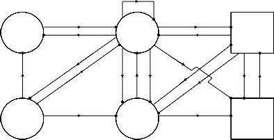
S5 ) of the system along with failure and repair rates against
By using simple probabilistic arguments, we have
the possible transitions are shown in the transition diagram
Q01 ( t ) = (1 − q
t +1 )
(Fig.1). In view of the discrete distributions involved, the sto- chastic model under study leads to the discrete parametric Markov-Chain with state space (S0 , S1 ,S2 ,S3 ,S4 ,S5 ) .
![]()
Q ( t ) = bqr 1 − ( bqs )
10 (1 − bqs )
bpr
t +1}
t +1
System initially starts from state S0 where one unit is op- erative and the other identical unit is kept into cold standby.
Q11
Q12
![]()
( t ) = (1 − bqs ) {1 − ( bqs ) }
![]()
( t ) = a (qs + pr ) 1 − ( bqs )t +1
(1 − bqs )
IJSER © 2014 http://www.ijser.org
International Journal of Scientific & Engineering Research, Volume 5, Issue 2, February-2014 923
ISSN 2229-5518
TRANSITION DIAGRAM
pr
No , Ns
RMg
p S1
Fr , No
RMo
p S3
Fr , Fw
RMo
ar ap
c cp apr c a cp a c ar
No , Ns
RMr
p p
Fw , No
RMr
Fw , Fw
RMr
![]()
![]()
![]()
: Up State : Failed State : Regenerative Point
Q13
![]()
( t ) = bps 1 − ( bqs ) (1 − bqs )
t +1}
Fig.1
p01 = p53
= 1 ,
p10
![]()
= bqr
(1 − bqs )
Q14
![]()
( t ) = aqr 1 − ( bqs ) (1 − bqs )
t +1}
p11
![]()
= bpr ,
(1 − bqs )
p12
a (qs + pr )![]()
=
(1 − bqs )
Q15
![]()
( t ) = aps 1 − ( bqs ) (1 − bqs )
t +1}
p13
![]()
= bps ,
(1 − bqs )
p14
![]()
= aqr
(1 − bqs )
Q21
![]()
( t ) = cq 1 − (dq ) (1 − dq )
t +1}
p15
![]()
= aps ,
(1 − bqs )
p21
![]()
= cq
(1 − dq )
![]()
Q ( t ) = cp 1 − (dq )
23 (1 − dq )
![]()
Q ( t ) = dp 1 − (dq )
25 (1 − dq )
t +1}
t +1}
p23
p31
![]()
= cp ,
(1 − dq )
![]()
= br ,
(1 − bs )
p25
p32
![]()
= dp
(1 − dq )
![]()
= ar
(1 − bs )
![]()
Q ( t ) = br 1 − ( bs )
31 (1 − bs )
ar
t +1}
t +1
p35
p
![]()
= as ,
(1 − bs )
= cp ,
p40
p
![]()
= cq
(1 − dq )
![]()
= dp
![]()
Q32 ( t ) = (1 − bs ) {1 − ( bs ) }
![]()
41 (1 − dq )
42 (1 − dq )
Q35
![]()
( t ) = as 1 − ( bs ) (1 − bs )
t +1}
We observe that the following relations hold-
p01 = p53 = 1
p + p + p
+ p + p + p = 1
cq t +1
10 11 12 13 14 15
![]()
Q ( t ) = (1 − dq ) {1 − (dq ) }
p + p + p = 1
40
cp t +1
21 23 25
p31 + p32 + p35 = 1
![]()
Q ( t ) = (1 − dq ) {1 − (dq ) }
p + p + p = 1
(18 − 22)
41
Q42
![]()
( t ) = dp 1 − (dq ) (1 − dq )
t +1}
40 41 42
( ) (
t +1 )
( ) Let
ψi be the sojourn time in state Si
(i = 0, 1, 2, 3, 4, 5)
Q53 t
= 1 − d
1 − 17
then mean sojourn time in state
Si is given by
The steady state transition probabilities from state Si
to Sj ∞
can be obtained from (1 − 17 ) by taking t →∞ as follows:
ψi = ∑ P [T ≥ t ]
t =1
In particular,
IJSER © 2014 http://www.ijser.org
International Journal of Scientific & Engineering Research, Volume 5, Issue 2, February-2014 924
ISSN 2229-5518
![]()
ψ = q ,
0 p
![]()
ψ = bqs
1 (1 − bqs )
+q35 ( t − 1) A5 ( t − 1)
( ) ( ) ( ) ( ) ( ) ( )
A4 t
= Z t
+ q40
t − 1 A0
t − 1 + q41
t − 1 A1
t − 1
ψ2 = ψ4 =
dq
![]()
(1 − dq )
= ψ (say)
+q42 ( t − 1) A2 ( t − 1)
( ) ( ) ( ) ( )
![]()
ψ = bs ,
ψ = d
( 23 − 27 )
A5 t
Where,
= q53
t − 1 A3
t − 1
32 − 37
![]()
3 (1 − bs ) 5 c
The values of Zi ( t ) ; i = 0, 1 and Z ( t ) are same as given in section 6(a).
In order to obtain various interesting measures of system
Let
m ( ) r
effectiveness we develop the recurrence relations for reliabil-
Bi t and
Bi ( t )
be the respective probabilities that
ity, availability and busy period of repairman as follows-
the repairman is busy at epoch (t-1) in the repair of RM and
units, when system initially starts from
Si . Using simple
probabilistic arguments as in case of reliability, the recurrence
Here we define
R i ( t )
as the probability that the system
relations for
j ( )
Bi t ; i = 0 to 5 can be easily developed as below.
does not fail up to t epochs 0, 1, 2,….,(t-1) when it is initially started from up state Si . To determine it, we regard the failed
The dichotomous variable δ takes values 1 and 0 respectively for j = m and r.
states S3 and S5 as absorbing states. Now, the expressions for
B j ( t ) = q
( t − 1) B j ( t − 1)
R i ( t ) ; i = 0, 1, 2, 4; we have the following set of convolution
0 01 1
j ( ) ( ) ( ) ( )
j ( )
B1 t
= 1 − δ Z1
t + q10
t − 1 B0
t − 1
equations.
( ) j ( ) ( )
j ( )
t −1
+q11
t − 1 B1
t − 1 + q12
t − 1 B2
t − 1
R ( t ) = q t +
∑ q01 ( u ) R1
( t − 1 − u )
+q ( t − 1) B j ( t − 1) + q
( t − 1) B j ( t − 1)
u =0
= Z0 ( t ) + q01 ( t − 1) R1 ( t − 1)
13 3 14 4
+q15 ( t − 1) B5 ( t − 1)
Similarly,
j ( ) ( ) ( )
j ( ) ( )
j ( )
R1 ( t ) = Z1 ( t ) + q10 ( t − 1) R 0 ( t − 1) + q11 ( t − 1) R1 ( t − 1)
B2 t
= δZ t
+ q21
( )
t − 1 B1
j ( )
t − 1 + q23
t − 1 B3
t − 1
+q25
t − 1 B5
t − 1
+q12 ( t − 1) R 2 ( t − 1) + q14 ( t − 1) R 4 ( t − 1)
j ( ) ( ) ( ) ( )
j ( )
B3 t
= 1 − δ Z3
t + q31
t − 1 B1
t − 1
R 2 ( t ) = Z2 ( t ) + q21 ( t − 1) R1 ( t − 1)
( ) j ( ) ( )
j ( )
+q32
t − 1 B2
t − 1 + q35
t − 1 B5
t − 1
R 4 ( t ) = Z4 ( t ) + q40 ( t − 1) R 0 ( t − 1) + q41 ( t − 1) R1 ( t − 1)
j ( ) ( ) ( )
j ( ) ( )
j ( )
+q42 ( t − 1) R 2 ( t − 1)
( 28 − 31)
B4 t
= δZ t
+ q40
( )
t − 1 B0
j ( )
t − 1 + q41
t − 1 B1
t − 1
Where,
+q42
t − 1 B2
t − 1
( ) t t t
t t B j ( t ) = δZ
( t ) + q
( t − 1) B j ( t − 1)
(38 − 43)
Z1 t
= b q s ,
Z2 ( t ) = Z4 ( t ) = d q
= Z ( t )
5 5 53 3
Where,
Let Ai ( t ) be the probability that the system is up at epoch
and
Z1 ( t )
and
Z ( t )
have the same values as in section 6(a)
(t-1), when it initially starts from state
Si . By using simple
Z3 ( t ) = b s ,
Z5 ( t ) = d .
probabilistic arguments, as in case of reliability the following recurrence relations can be easily developed for Ai ( t ) ; i = 0 to
5.
A0 ( t ) = Z0 ( t ) + q01 ( t − 1) A1 ( t − 1)
A1 ( t ) = Z1 ( t ) + q10 ( t − 1) A0 ( t − 1) + q11 ( t − 1) A1 ( t − 1)
Taking geometric transforms of (28-31) and simplifying the resulting set of algebraic equations for R* ( h ) , we get
+q12 ( t − 1) A2 ( t − 1) + q13 ( t − 1) A3 ( t − 1)
+q14 ( t − 1) A4 ( t − 1) + q15 ( t − 1) A5 ( t − 1)
A2 ( t ) = Z ( t ) + q21 ( t − 1) A1 ( t − 1) + q23 ( t − 1) A3 ( t − 1)
Where,
R* ( h ) =
N1 ( h )
![]()
D1 ( h )
( 44)
+q25 ( t − 1) A5 ( t − 1)
N ( h ) = 1 − hq*
− hq*
(hq*
+ h 2 q* q*
) − h 2 q* q* Z*
1 11 21 12 14 42 14 41 0
A3 ( t ) = q31 ( t − 1) A1 ( t − 1) + q32 ( t − 1) A2 ( t − 1)
* * * ( * *
2 * * ) *
+hq01Z1 + hq01
hq12 + hq14 + h q14 q42 Z
IJSER © 2014 http://www.ijser.org
International Journal of Scientific & Engineering Research, Volume 5, Issue 2, February-2014 925
ISSN 2229-5518
( )
* * ( *
2 * * )
2 * *
( ) ( ) ( )}
D1 h
= 1 − hq11 − hq21
hq12 + h q14 q42
− h q14 q41
p12 + p14 p42
+ p32
p13 + p15
+ p14
p31 + p32 p21 ψ
2 * *
3 * * *
+ {(1 − p21 ) ( p12 + p14 p42 ) + ( p13 + p15 )}ψ3
−h q01q10 − h q01q14 q40
Collecting the coefficient of h t
from expression (44), we
+ {( p35 + p32 p25 ) ( p12 + p13 + p15 + p14 p42 ) − ( p12
can get the reliability of the system R 0 ( t ) . The MTSF is given
by-
+p14 p42 ) − ( p21p35 + p31p25 ) + p15 ( p31 + p32 p21 )}ψ5
Now the expected up time of the system up to epoch (t-1) is
E (T )
∞ N (1)
![]()
= lim ∑ h t R ( t ) = 1 − 1
( 45)
given by
h →1 t =1
D1 (1)
µup
( t )
t −1
= ∑ A0
( x )
N1 (1) = 1 − p11 − p21 ( p12 + p14 p42 ) − p14 p41 ψ0
+ψ1 + p12 + p14 (1 + p42 ) ψ
so that
* ( )
x =0
![]()
* ( ) ( )
D1 (1) = 1 − p11 − p21 ( p12 + p14 p42 ) − p14 p41 − p10 − p14 p40
µup h
= A0
h 1 − h
( 48)
On taking geometric transform of (32-37) and simplifying
On taking geometric transforms of (38 − 43)
and simpli-
the resulting equations, we get
fying the resulting equations for j = m and r, we get
Bm* h
N ( h )
![]()
= 3
and
Br* ( h ) = N4 ( h )
( 49 − 50)
![]()
A* ( h ) = N2 ( h )
( 46)
0 ( ) ( )
![]()
0 ( )
0
Where,
( ) {
D2 ( h )
2 * * * ( *
2 * * )}{ 2
* * *
Where,
( )
D2
* (
h
2 * * )( * *
D2 h
2 * * )
N2 h
= 1 − h q35q53 − hq32
hq23 + h q25q53
h q01q14 Z
N3 h
= hq01 1 − h q35 q53
hq12 + hq14 + h q14 q42
+ 1 − hq11 − h q14 q41
Z0 + hq01Z1
+hq32 {(hq13 + h q15 q53 ) − hq14 (hq23 + h q25 q53 )} Z
( * 2
* * ) *
* *}
* * 2
* * * *
2 * * *
+ 1 − h q35q53
hq12 + h q14 q42
+ hq32
hq13
+hq01 {(hq15 + h q13q35 ) + hq14 (h q42 q25 +h q23q35 q42 )
{( 2
* * )( *
2 * * )
* ( *
* * 2
* * *
2 * *
3 * * *
+h q15 q53
hq01Z
− hq21Z0
− hq31
hq13
+hq12 (h q23q35 + hq25 ) + hq32 (h q13q25 − h q15 q23 )} Z5
2 * * )}(
* * * * )
* { *
* 2 * * * *
2 * *
2 * * *
+h q15 q53 +
hq23 + h q25q53
hq12 + h q14 q42 Z0
N4 ( h ) = hq01 {1 − h q35q53 − hq32 (hq23 + h q25q53 )} Z1 + {(hq13
2 * * ( *
2 * * )( *
2 * * )} *
* 2
* * * *
2 * * * *
( ) {
* 2 * *
2 * * 3 * * * }
2 * * ) ( *
2 * * )( *
2 * * )} *
D2 h
= 1 − hq11 − h q14 q41 − h q01q10 + h q01q14 q40
+h q15 q53
+ hq23 + h q25 q53
hq12 + h q14 q42 Z3
{ 2 * * * ( *
2 * * )}
and D h is same as in availability analysis.
1 − h q35q53 − hq32
hq23 + h q25q53
2 ( )
{( 2
* * )( *
2 * * )
* ( *
In the long run, the respective probabilities that the re-
− 1 − h q35q53
hq12 + h q14 q42
+ hq32
hq13
pairman is busy in the repair of RM and units are given by-
2 * * )}(
2 * * * )
* { *
Bm = lim Bm ( t ) = lim (1 − h ) N3 ( h )
+h q15 q53
h q01q20 + hq21
− hq31
hq13
![]()
0 t →∞ 0
h →1 D2
( h )
2 * * ( *
2 * * )( *
2 * * )} N h
+h q15 q53 +
hq23 + h q25q53
hq12 + h q14 q42
Br = lim Br ( t ) = lim (1 − h )
![]()
4 ( )
The steady state availability of the system is given by-
0 t →∞ 0
h →1
D2 ( h )
A = lim A
![]()
( t ) = lim (1 − h ) N2 ( h )
But
D2 ( h )
at h=1 is zero, therefore by applying L. Hospital
0 t →∞ 0
h →1
D2 ( h )
rule, we get
As D2 ( h )
at h=1 is zero, therefore by applying L. Hospital![]()
Bm = − N3 (1)
and![]()
Br = − N4 (1)
(51 − 52)
rule, we get
A
N2 (1)
= −
( 47 )
0
Where,
D′2 (1)
D′2 (1)![]()
0 D′ (1)
( ) {( ) ( ) ( ) (
2 N3 1 =
1 − p35
p12 + p14 p42
+ p32
p13 + p15
+ p14
p31
Where,
N2 (1) = ( p31 + p32 p21 ){( p10 + p14 p40 ) ψ0 + ψ1} + {(1 − p35 )
+p32 p21 )}ψ+ {( p35 + p32 p25 ) ( p12 + p13 + p15 + p14 p42 )
( ) ( ) ( )}
+p15
p31 + p32 p21
− p12 + p14 p42
p21p35 + p31p25 ψ5
( p12 + p14 p42 ) + p32 ( p13 + p15 ) + p14 ( p31 + p32 p21 )}ψ
( ) ( )
{( ) ( )
and
N4 1 =
p31 + p32 p21
ψ1 +
1 − p21
p12 + p14 p42
D′2 (1) = ( p31 + p32 p21 ){( p10 + p14 p40 ) ψ0 + ψ1} + {(1 − p35 )
+ ( p13 + p15 )}ψ3
IJSER © 2014 http://www.ijser.org
International Journal of Scientific & Engineering Research, Volume 5, Issue 2, February-2014 926
ISSN 2229-5518
and D′2 (1) is same as in availability analysis.
The expected busy periods of the repairman in the repair of RM and units up to epoch (t-1) are respectively given by-
t −1
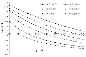
Similarly, fig. 3 reveals the variations in profit (P) with re- spect to p for varying values of r and c, when the values of other parameters are kept fixed as a = 0.6, K₀=150, K₁=100 and K₂=80. From the curves we observe that profit decreases uni-
µb ( t ) =
∑ B0 ( x )
formly as the values of p increase. It also reveals that the profit
x =0
t −1
b ∑ 0
increases with the increase in r and increases with the increase
in c. From this figure it is clear from the dotted curves that the
So that,
µr ( t ) =
Br ( x )
x =0
system is profitable only if failure rate (p) is greater than 0.06,
0.11 and 0.17 respectively for r = 0.3, 0.5, and 0.7 for fixed val-
ue of c = 0.075. From smooth curves, we conclude that the sys-
m* ( h ) =
![]()
m* ( h )
(53)
tem is profitable only if p is greater than 0.78, 0.14 and 0.21 respectively for r = 0.3, 0.5, and 0.7 for fixed value of c = 0.10.
(1 − h )
µr* ( h )
b
r* ( h )
![]()
=
(1 − h )
(54) Behaviour of MTSF with respect to p, r and c
We are now in the position to obtain the net expected profit incurred up to epoch (t-1) by considering the character- istics obtained in earlier sections.
Let us consider,
K0 = revenue per-unit time by the system when it is oper- ative.
K1 = cost per-unit time when repairman is busy in the re-
pair of the failed RM.
K 2 = cost per-unit time when repairman is busy in the re- pair of the failed units.
Then, the net expected profit incurred up to epoch (t-1) is giv-
en by
P ( t ) = K µ
( t ) − K µm ( t ) − K µr ( t )
(55)
0 up 1 b 2 b
The expected profit per unit time in steady state is as follows-
P ( t )
![]()
P = lim
t →∞
t
( )2 A
( h )
m*
( )2 0
( h )
![]()
= K0 lim 1 − h
h →1
0
(1 − h )
![]()
− K1 lim 1 − h
h →1
(1 − h )
r*
![]()
−K lim (1 − h )2 0
( h )
= K0 A0 − K1B0 − K 2 B0
h →1
(1 − h )
(56)
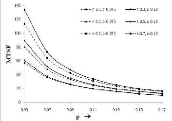
The curves for MTSF and profit function have been drawn for different values of parameters p, r, c. Fig. 2 depicts the var- iations in MTSF with respect to failure rate (p) of an operative unit for different values of repair rate (r = 0.3, 0.5, 0.7) of a failed unit and the failure rate (c = 0.075, 0.10) of RM. From the curves we observe that MTSF decreases uniformly as the val- ues of p increase. It also reveals that the MTSF increases with the increase in r and increases with the increase in c.
1. B. S. Dhillon, H. C. Vishvanath, “Reliability analysis of a non-identical unit parallel system with common cause
failure”, Microelectron Reliab., Vol. 31, pp. 429-441 (1991).
IJSER © 2014 http://www.ijser.org
International Journal of Scientific & Engineering Research, Volume 5, Issue 2, February-2014 927
ISSN 2229-5518
2. L.R Goel, R. Gupta, S.K. Singh, “Cost-benefit analysis of a two-unit warm standby system with inspection, repair and post-repair” IEEE Transaction on Reliability, Vol. R
35, No. 1, pp. 70 (1986).
3. V. Goyal, K. Murari, “Optimal policies in a two-unit standby system with two types of repairmen”, Microelec- tron reliability, Vol. 24, No. 5, pp. 857-864 (1984).
4. R. Gupta, Shivakar, “A two non identical unit parallel system with waiting time distribution of repairman” Int. J. of management and system, Vol. 100, No. 1, pp. 77-90 (2003).
5. R. Gupta, A. Chaudhary, “Analysis of stochastic models in manufacturing systems pertaining to repair machine failure”, C.R.C. (2001).
6. R. Gupta, A. Chaudhary, “Cost-bebefit analysis of a two unit standby system with provision of repair machine failure,” Microelectron Reliab. Vol. 34, No. 8, pp. 1891-
1394 (1994).
7. A.K. Mogha, R. Gupta, A.K. Gupta, “A two priority unit warm standby system model with preparation for repair”, Aligarh J of Statistics, Vol. 22, pp.73-90 (2002).
8. A.K. Mogha, R. Gupta, A.K. Gupta, “A two-unit parallel
system with correlated lifetimes and repair machine fail- ure”, IAPQR, Vol. 28, No. 1, pp. 1-22 (2003).
9. S.K. Singh, B. Srinivasu, “Stochastic analysis of a two unit cold standby system with preparation time for repair”,
Microelectron reliability, Vol. 27, pp. 50-60 (1987).
IJSER © 2014 http://www.ijser.org