International Journal of Scientific & Engineering Research, Volume 3, Issue 1, January-2012 1
ISSN 2229-5518
A Simplified Pipeline Calculations Program: Liquid Flow (1)
Tonye K. Jack
Abstract— and Program Objective - A multi-functional single screen desktop companion program for piping calculations using Microsoft EXCELTM with its Visual basic for Applications (VBA) automation tool is presented. The program can be used for the following piping geometries – circular, rectangular, triangular, square, elliptical and annular. Fluid properties are obtained from built-in fluid properties functions.
Index Terms— engineered spreadsheet solutions, liquid pipline flow, pipeline design, pipeline fluid properties, piping program, pipeline sizing.
—————————— ——————————
HE piping designer will often be saddled with the task of designing for different pipe configurations (circular, square ducts, etc.). Conducting such piping designs, can often involve repetitive calculations whether for simple hori-
Head Loss:
h f
![]()
fLV 2
8 fLQ 2
![]()
(4)
zontal pipelines or piping of complex terrains. Modern com- puter- assisted - tools are now often employed as aids in achieving these, if time and cost permits. Often times, for mi- nor changes to existing installations or retrofitting, a customer
2gD
2 2
gD5
(pipeline owner) would contract an engineering consultancy
to conduct an analysis check that will involve desktop routine
calculations such as determining pressure drops, or head loss,
flow rate or pipe geometry (diameter, length, cross-sectional
area, etc.) that can be assigned to an engineer for quick an-
swers. Simple spreadsheet calculators can be developed to aid
such small routine calculations. One such program is shown
Friction Factor: The friction factor, f, is obtained as follows:
For Laminar Flow: The applicable equations for laminar flows (Re≤2100) can be defined in terms of a laminar flow factor, Lf, which varies depending on the pipe geometry. The equation is of the form:
here with all required equations to assist in developing one.
f .Re L f
(5)
For Turbulent Flow, the friction factor, f is obtained by the
Colebrook-White equation
Reynolds Number:![]()
1
![]()
![]()
1 2Log
2.51
![]()
(6)
Re
Flow Velocity:
VD
![]()
(1)
f 2
Flowrate:
3.7
e
Area:![]()
V Q A
D 2
![]()
A
4
(2)
(3)
For Laminar Flow:
gD4 h
![]()
Q f
128L
For Turbulent Flow:
Q VA
(7)
(8)
IJSER © 2012
International Journal of Scientific & Engineering Research, Volume 3, Issue 1, January-2012 2
ISSN 2229-5518
gD5 h
0.5
0.5
2
Also, for Turbulent Flow within the limits defined below, explicit values for the friction factor, f is obtained by the Swamee-Jain
Q
D2 f
![]()
Ln
3.17 L
relationship, ―(16),‖.
0.965
3.7D
gD3h
(9)
f 0.25Log
![]()
2
5.74
![]()
3.7
R 0.9
Range of application: 10-6 ≤ (ε/D) ≤ 2 x 10⁻²
3 x 10³ ≤ Re ≤ 3 x 10⁸
e
(16)
Solution for Diameter:
8 fLQ 2
5
Range of application: 10-6 ≤ (ε/D) ≤ 2 x 10⁻²
3 x 10³ ≤ Re ≤ 3 x 10⁸
D
gh f
4.75
0.04
(10)
The Microsoft Excel TM Solver Add-in, has two built-in interpo- lation search solution methods – the Newton method and the Conjugate Gradient method. By rewriting the equation to be
LQ2
L
solved in the solution form required (see ‚17,‛) in the Micro-
D 0.66 1.25
![]()
Q9.4
soft ExcelTM cells, the Solver Add-in option dialog box under
gh f
gh
the Tools menu, allows for desired constraints to be set as fol-
(11)
lows:
Range of application: 10-6 ≤ (ε/D) ≤ 2 x 10⁻²
3 x 10³ ≤ Re ≤ 3 x 10⁸
Pressure Drop
Set Target Cell: Equal To:
Subject to: Guess value:
P hf
ghf
g
![]()
(12)
![]()
![]()
1 2Log D
1 3.7
2.51
f R
0
(17)
Shear Stress in Wall:![]()
f 2
e
f V 2
![]()
![]()
4 2g
The Microsoft ExcelTM Goal Seek option is also useful.
Furthermore, the solution method provides for limiting the number of iterations, the degree of precision desired and the
(13)
level of convergence (i.e. the decimal floating points). The er-
ror margin involved in the iteration calculation is indicated by
Power required to pump through the line:
the Tolerance percentage. Care should be exercised to avoid a risk of having a circular reference – repeated recalculation of
Pw Qhf
Qghf
(14)
particular cell values as input and output.
The Laminar Flow factor is defined by the relation:
Lf = Laminar Flow factor = f. Re = 64 (15)
For Turbulent Flow, f, is obtained by the Colebrook-White for- mula, ―(6),‖.
Miller [1], suggest that a single iteration will produce a result within 1% of the Colebrook-White formula, if the initial esti- mate is calculated from the Swamee-Jain equation.
In determining the flow regime and velocity gradients in a pipeline, the wetted perimeter (the perimeter in contact with the fluid) is the consideration. For non-circular pipes, the Rey- nolds number is a function of a concept called a hydraulic Di-
IJSER © 2012
International Journal of Scientific & Engineering Research, Volume 3, Issue 1, January-2012 3
ISSN 2229-5518
ameter, defined as the ratio of the cross-sectional area of the piping section to the wetted perimeter.
The hydraulic diameter is defined such that it reduces to the diameter for the circular pipes (Cengel et. al., ‚[2],‛). It is gen- erally a parameter for generalising fluid flow in turbulent flow. The hydraulic diameter concept does not apply for lami- nar flow through non-circular pipe sections. The hydraulic
diameter for different piping configurations is provided by
Engineering Sciences Data Unit (ESDU), [3], [4].
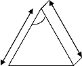
Fig 2: geometry of isosceles triangular pipe section
Source: [3], [4]
The laminar flow factors vary as a function of the isosceles angle, in line with the values in Table 1.
Note that angles falling between those in the table can be ob- tained by straight line interpolation.
Table 1: Laminar flow factors for Isosceles duct type pipes
Source: ESDU, [3], [4]
D
D
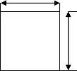
Fig. 1: geometry of square pipe section- Source: [3], [4]
A = D2 (17) Dh = D = hydraulic diameter (18)
For laminar flow, ‚(5)‛, is applied, as follows,
Lf = Laminar Flow factor = f.Re = 14.2 (19)
![]()
 d
d
![]()
D
Thus,
14.2
Fig 3: geometry of Rectangular pipe section-Source: [3], [4]![]()
f (19a)
Re
A Dd
(22)
A ½d 2 sin
(20)
![]()
D 2Dd
h D d
(23)
Dh
d sin
(21)
d
d
![]()
1 sin
![]()
f .Re 160.67 0.46
![]()
2
2 D
D
(24)
The Laminar flow factor, (f.Re) is defined in terms of the (D/d)
d d ratio by ‚(24),‛
θ
The Variation of Laminar Flow factors for different (D/d) val- ues is as shown in Table 2.
IJSER © 2012
International Journal of Scientific & Engineering Research, Volume 3, Issue 1, January-2012 4
ISSN 2229-5518
Again, duct side ratios falling between those in the table can
be obtained by straight line interpolation.
Table 2: Laminar flow factors for Rectangular duct type pipes
Source: ESDU, [3], [4]
Laminar flow factors for triangular pipe sections of the right-
angled type, for variations in the angle θ¸ defined by ‚(31),‛ is shown in Table 3.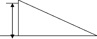
Again, angles falling between those in the table can be ob- tained by straight line interpolation.
d
θ
![]()
D
Fig 5: geometry of right-angled triangular pipe section
Source: [3], [4]
![]() 2d
2d
2D Dh ![]()
A dD
2
2dD
(30)
(29)![]()
d
D d 2
D2 0.5
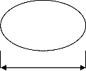
Fig 4: geometry of elliptical pipe section- Source: [3], [4]
d
![]()
tan 1
(31)
A Dd
(25)
D
Hydraulic diameter,
4Dd 64 16c2
![]()
Dh d D64 3c4
Where, for, 0.1 < (D/d) < 10
D d
Table 3: Laminar flow factors for Right-angled duct type pipes
Source:ESDU, [3], [4]
(2
c D d
(27)
The Laminar flow factor for elliptical pipe sections is obtained from ‚(28),‛.
2D 2 D 2 d 2
Microsoft ExcelTM Functions category (under the Insert menu
option) can be used to develop a database of mouse click, drop-down physical properties of typical pumping liquids. Y(aws, [5], [6], [7], [8], provides density, viscosity, and vapour
f .Re
![]()
d 2 D 2
28)
pressure data as a function of temperature in line with the
mathematical relation, function(Temperature), i.e ƒ(T).
For example, [8], derived general curve-fitted density relation- ships for certain fluid types as functions of reduced tempera- ture. As an example, for Chlorobenzene (C6H6Cl), the follow-
ing relations for liquid density apply:![]()
2
L AB
IJSER © 2012
1Tr
(32)
International Journal of Scientific & Engineering Research, Volume 3, Issue 1, January-2012 5
ISSN 2229-5518
Where the constants are: A= 0.3706, B= 0.2708
Tr is the reduced temperature = T/Tc
Tc = Critical temperature of Chlorobenzene = 359.2oC
The constant terms vary from one fluid type
to another.
The liquid density value is in g/cm3. Conversion to kg/m3 can
be made in the program by multiplying by 1000.
When developing a fluid properties function data pack in Mi- crosoft ExcelTM, it is recommended to follow a structured nam- ing convention to allow for an error free process in selection using the drop-down list button. One useful method given by ALIGNAgraphics [9], is:
Name of property_ (temperature)
For water: rhoWater(temperature)
Where rhoWater, and viscWater are the function names for water density and Liquid viscosity respectively.
Writing the VBA Module Function code procedure, for exam- ple for Chlorobenzene liquid density using ‚(32),‛ is of the form:
Function rhoChlorobenzene (temperature)
Tr=T/359.2 ‘returns reduced temperature value’ C=(-(1-Tr))^(2/7) ‘returns the exponent value’ rhoChlorobenzene=(0.3706)*(0.2708)^C
End Function
Compared to a VBA subroutine (SUB) procedure, a FUNC- TION procedure has a return value. Thus, by entering the function procedure name into a cell, a return value can be ob- tained by referencing the function dependent cell. In this case the functions are dependent on temperature.
The Excel worksheet screen shot shown in Fig. 10 shows link
cells with the built in Excel developed formulae. The Interface Excel screen is formatted using the Excel VBA icons which are directly pasted on the sheet. The outputs obtainable for differ- ent piping parameter inputs are displayed using the VBA Worksheet subroutine macros shown in the program clip of the Appendix.
Example 1: Circular Pipes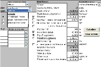
Water at 20 oC flows through a cast iron pipe at the rate of 1.2 m3/s. The pipe is 340 m long and the head loss through the line is 80 m. What size pipe is required? Also determine the power lost to friction, the pressure drop and the shear rate in the wall?
Fig. 5: A clip of Excel Screen Solution for the Example 1
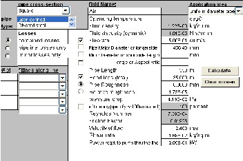
Example 2: Square Pipe Cross-section
A 350 m long square cross-section duct is used to transport air. Evaluate the pipeline given the following? Take that: Pipe Roughness = 0.008 mm; Air density = 1.22 kg/m3; Viscosty =
1.81 x 10
N.s/m , headloss = 35 m; flow rate = 0.5 m /s.
-5 2 3
IJSER © 2012
International Journal of Scientific & Engineering Research, Volume 3, Issue 1, January-2012 6
ISSN 2229-5518
Example 4: Elliptical Ducts
A galvanized pipe, elliptical cross-section of 2:1 aspect ratio is used to transport water at 15oC at the rate of 0.2 m3/s through a
150 m line. If head loss is 23 m, evaluate the pipeline?
Fig. 8: A clip of Excel Screen solution for the Example 4
Fig 6: A clip of Excel Screen Solution for the Example 2
Example 3: Triangular Ducts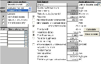
A 40 m long triangular conduit made of commercial steel is used to carry water at 20 oC, at the rate of 0.3 m3/s. If the head loss is 4 m, and the triangular section is shaped in the form of an isosceles triangle with ¸=35o, find the length of the longest side, x?
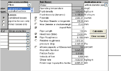
Example 5: Circular pipe with fittings along line
Ethanol at 20 oC flows from tank 1 to tank 2 at the rate of 0.024 m3/s through a 100 mm-diameter, 100 m long pipe. Compute the total head loss, if the fittings along the pipe include a 90o Long Radius Elbow, and a gate valve. (ε/D=0.00065)
pipe cross-section fluid Name: Application area
circular Ethanol uniform diameter pipeline
pipe Operating temperature 20 degC
type: user-defined Fluid density 7.98E+02 kg/cu.m Losses Fluid viscosity (dynamic) 1.14E-03 N.s/sq.m combined losses Flowrate 2.40E-02 cu.m/s pipeline losses only Pipe Major Diameter or longerside 100.00 mm
minor losses only Minor Diameter or shortside-length mm
angle or Aspect ratio
# of fittings along line Pipe Length 100 m
1 90 deg long radius elbow Head loss (total) 314.735 m
1 Gate valve, fully open Pipe Roughness 0.0650 mm
0 Relative roughness 6.50E-04
0 pressure drop 2.46E+06 Pa
0 efficiency(specify or 100assumed) 100 percent
Reynolds Number 2.14E+05
Friction Factor 0.01945
Velocity of flow 3.056 m/s Shear rate 1.81E+01 kg/sq.m Power reqd. to pump thru the line 5.92E+01 kW
R © 2012
ww.ijser.org
International Journal of Scientific & Engineering Research, Volume 3, Issue 1, January-2012 7
ISSN 2229-5518
ElseIf 2 <= ActiveSheet.Range("M13") And ActiveSheet.Range("M13") <=
10 Then
ActiveSheet.Range("F13") = ActiveSheet.Range("Q17") End If
End Sub
![]()
Nomenclature
P1 Upstream pressure (kPa).
P2 Downstream pressure (kPa ).
Pw Power Required (kW)
Q Flowrate (KN/s).
g Gravity constant (m/s2).
hf Head loss (m or J/kg)
A Area (m2).
f Friction factor
D Pipe Major or Minor diameter (m)
Dh Hydraulic diameter (m)
L Pipe section length (m).
V Velocity of flow (m/s).
ε Pipe Rougness (mm)
γ Specific weight (kN/m3).
ρ liquid density (kN-s2/m4).
τ Shear rate
A Clip of Microsoft Excel VBA Cells – Link Worksheet Subroutines for
Display Interface
Sub pipeType()
If ActiveSheet.Range("M13") = 1 Then
ActiveSheet.Range("F13") = ""
'Perform pipe sizing calculations
'Circular pipeline section calculations
Sub circular()
Rho = ActiveSheet.Range("F5") visc = ActiveSheet.Range("F6") D = ActiveSheet.Range("F8")
d1 = ActiveSheet.Range("F9") AspectAngle = ActiveSheet.Range("F10") L = ActiveSheet.Range("F11")
'pipe sizing for circular section given relative roughness, headloss un- known
If ActiveSheet.Range("M17").Value = 2 And (Active- Sheet.Range("M6").Value = 1 Or ActiveSheet.Range("M6").Value = 2 Or ActiveSheet.Range("M6").Value = 3) And ActiveSheet.Range("M9").Value
= True And ActiveSheet.Range("M10").Value = True And Active- Sheet.Range("M15").Value = 1 Then
ActiveSheet.Range("F13") = ActiveSheet.Range("R17") ActiveSheet.Range("F19") = ActiveSheet.Range("R23") ActiveSheet.Range("F17") = ActiveSheet.Range("R28") Sheets("incompressible flow").Range("R11").GoalSeek Goal:=0, Chan-
gingCell:=Sheets("incompressible flow").Range("R7") ActiveSheet.Range("F18") = ActiveSheet.Range("R29") ActiveSheet.Range("F12") = ActiveSheet.Range("R25") ActiveSheet.Range("F20") = ActiveSheet.Range("R30") ActiveSheet.Range("F21") = ActiveSheet.Range("R31") ActiveSheet.Range("F16") = ActiveSheet.Range("R32") ActiveSheet.Range("F15") = ActiveSheet.Range("R33")
'same as above but given PipeRoughness not relative roughness
ElseIf ActiveSheet.Range("M17").Value = 2 And (Active- Sheet.Range("M6").Value = 1 Or ActiveSheet.Range("M6").Value = 2 Or ActiveSheet.Range("M6").Value = 3) And ActiveSheet.Range("M9").Value
= True And ActiveSheet.Range("M10").Value = True And Active- Sheet.Range("M15").Value = 2 Then
ActiveSheet.Range("F14") = ActiveSheet.Range("S18") ActiveSheet.Range("F19") = ActiveSheet.Range("S23") ActiveSheet.Range("F17") = ActiveSheet.Range("S28") Sheets("incompressible flow").Range("S11").GoalSeek Goal:=0, Chan-
gingCell:=Sheets("incompressible flow").Range("S7") ActiveSheet.Range("F18") = ActiveSheet.Range("S29") ActiveSheet.Range("F12") = ActiveSheet.Range("S25") ActiveSheet.Range("F20") = ActiveSheet.Range("S30") ActiveSheet.Range("F21") = ActiveSheet.Range("S31") ActiveSheet.Range("F16") = ActiveSheet.Range("S32") ActiveSheet.Range("F15") = ActiveSheet.Range("S33")
'pipe sizing for circular section given relative roughness diameter un- known
ElseIf ActiveSheet.Range("M17").Value = 2 And (Active- Sheet.Range("M6").Value = 1 Or ActiveSheet.Range("M6").Value = 2 Or ActiveSheet.Range("M6").Value = 3) And ActiveSheet.Range("M9").Value
= True And ActiveSheet.Range("M11").Value = True And Active- Sheet.Range("M15").Value = 1 Then
ActiveSheet.Range("F13") = ActiveSheet.Range("T17")
End If
IJSER © 2012
International Journal of Scientific & Engineering Research, Volume 3, Issue 1, January-2012 8
ISSN 2229-5518
End Sub
[1] R. W. Miller, Flow Measurement Engineering Handbook, 1985, (McGraw-Hill)
[2] Y. A. Cengel, R. H. Turner, and Cimbala, Fundamentals of Thermal - Fluid Sciences, 3rd edn., McGraw-Hill, 2008
[3] Engineering Sciences Data Unit, Friction Losses for fully developed flow in straight pipes, ESDU 66027
[4] Engineering Sciences Data Unit, Friction Losses for fully developed flow
in straight pipes of constant cross –section – subsonic compressible flow of gases, ESDU 74029
[5] C. L. Yaws., “Correlation constants for Chemical Compounds”,
Chemical Engineering, Aug. 16, 1976, pp. 79-87
[6] C. L. Yaws., “Correlation constants for Liquids”, Chemical Engineer- ing, Oct.25, 1976, pp.127-135
[7] C. L. Yaws, “Correlation constants for Chemical Compounds”,
Chemical Engineering, Nov. 22, 1976, pp.153-162
[8] C. L. Yaws., “Physical Properties”, 1977, (McGraw Hill)
[9] AlignaGraphics Co., UK, “Pipeline Sizing Program”, Pipedi User Ma- nual, 1998
[10] J. B. Evett, 2500 Solved Problems in Fluid Mechanics & Hydraulics 1989,
(McGraw-Hill)
[11] A. Esposito, Fluid Power with Applications, 1980, (Prentice Hall) [12] R. N. Fox, Introduction to Fluid Mechanics, 1992, (Wiley)
[13] L. F. Moody, “Friction Factors for Pipe Flow “, Trans. ASME, Vol. 66, No. 8, pp. 671, 1944
[14] P. K. Swamee, A. K. Jain, “Explicit Equations for Pipe Flow Prob-
lems“ Journal of Hydraulic Division, Proc. ASCE, pp. 657-664., May,
1976
[15] W. L. McCabe, J. C. Smith, and P. Harmott, Unit Operations in Chemi- cal Engineering, 4th edn, pp. 91-92, 1985, (McGraw-Hill)
[16] R. H. Perry, and D. W. Green, (eds), Perry’s Chemical Engineers’ Hand- book, 6th edn, 1984, (McGraw Hill)
[17] V. L. Streeter, Fluid Mechanics, 1983, (McGraw-Hill)
BIOGRAPHICAL NOTES
T. K. Jack is a Registered Engineer, and ASME member. He worked on rotating equipment in the Chemical Fertilizer industry, and on gas tur- bines in the oil and gas industry. He has Bachelors degree in Mechanical Engineering from the University of Nigeria, and Masters Degrees in Engi- neering Management from the University of Port Harcourt, and in Rotat- ing Machines Design from the Cranfield University in England. He was the Managing Engineer of a UK Engineering Software Company, ALIG- Nagraphics and the developer of a Pipeline sizing program, “PipeDi”. He is a University Teacher in Port Harcourt, Rivers State, Nigeria, teaching undergraduate classes in mechanical engineering. He can be reached by
Email: - tonyekjack@yahoo.com
IJSER © 2012