International Journal of Scientific & Engineering Research Volume 3, Issue 8, August -2012 1
ISSN 2229-5518
*Ms. Sraboni Mandal, **Dr. Danish Ali Khan
![]()
![]()
A JELS probabilistic model developed for a single vendor multi customers situation where demand of the customers and stock level of the vendor are identically distributed random variables belonging to Weibulls Distribution.
A stochastic model differs
substantially from multi-customer policies of Lu Lu [39,(1995)] and Drenzer and Wesolowsky [13,(1989)]. But here technique of negotiation and pricing policies have been derived from the deterministic model of Banerji A[3, (1986)]. In this paper the model has been developed and has been illustrated through a numerical example.
Coordination between two different business entities is an important way to gain competitive advantage as it lowers supply chain cost. This paper reviews literature dealing with buyer vendor coordination models that have used quantity discount as coordination mechanism under deterministic environment and classified the various models. In a typical purchasing situation, the issues of price, lot sizing etc., usually are settled through negotiations between the purchaser and the vender. The effective ways for a compromise between one vender and multiple customers at a common lot size with certain amount of price adjustments are determined and the methodology is explained through a numerical example.
*Department of Computer Applications, Assistant Professor, National Institute of Technology, Jamshedpur, India, Email: man_sranitjsr@yahoo.com
** Department of Computer Applications, Assistant Professor , National Institute of Technology, Jamshedpur, India, Email: dakhan_nitjsr@sify.com
International Journal of Scientific & Engineering Research Volume 3, Issue 8, August -2012 2
ISSN 2229-5518
In the process, such a supply chain loses to supply chain that is customer focused where the individual links orient their business processes and decisions to ensure least cost delivery of products/services to the ultimate customer. Narasimhan and Carter (1998) in their work have mentioned that a well- integrated supply chain involves coordinating the flows of materials and information between suppliers, manufacturers, and customers. Thomas and Grifin (1996) have mentioned that effective supply chain management requires planning and coordination among the various channel members including manufacturers, retailers and intermediaries if any.
Several strategies are used to align the business processes and activities of the members of a supply chain to ensure better supply chain performance in terms of cost, response time, timely supply and customer service. Supply chain coordination is concerned with the development and implementation of such strategies. There is no universal coordination strategy that will be efficient and effective for all supply chains as the performance of a coordination strategy is supply chain characteristics dependent. Supply chain coordination through quantity discount has received much attention in Production/Operations Management literature only recently (Weng,
1995a,b). Since quantity discount is
considered to be one of the most popular mechanisms of coordination between the business entities, this paper primarily investigates supply chain coordination models that have used quantity discount as coordination tool under deterministic environment. However, we have also included here some integrated buyer vendor models that have similar type of objective function to achieve production distribution coordination and that improves the performance of the supply chain. In this
paper, the word vendor, supplier and manufacturer is used alternatively to represent the same upstream member in the supply chain who sells the item to the buyer unless specifically mentioned.
Many researchers like Monahan [1], Lee [2], Joglekar[4], have discovered various methods of discount polices to satisfy the vendor. This paper deals with a discount policy which causes no loss to both the parties and both are getting some benefit.
The following notation are used in developing the model.
I) i an integer such that 1≤ i ≤ n.
II) Ci represents the customer i.
III) Xi = Random demand (lot size) of the customer Ci (i=1,2,3,…..n)
Where,
fi(x) = ![]() , 0< x < ∞
, 0< x < ∞
if A = ![]() then
then
I = A ![]()
![]() dx where k > 0, λ > 0
dx where k > 0, λ > 0
IV) Y = The random inventory stock level (lot size) of the vendor, with density function f(y).
V) t = Scheduling time period which is a prescribed constant.
VI) Cv1 = Carrying cost (holding cost) of the vendor per unit item per t time units.
VII) Cv2 = Shortage cost (penalty) of the vendor per units item per t time units.
IJSER © 2012 http://www.ijser.org
International Journal of Scientific & Engineering Research Volume 3, Issue 8, August -2012 3
ISSN 2229-5518
![]()
VIII) = Carrying cost (holding cost) of
the customer Ci per unit item per t time units.
IX) ![]() = Shortage cost (penalty) of the customer Ci per unit item per t time units.
= Shortage cost (penalty) of the customer Ci per unit item per t time units.
X) Z = Variable lot size (i.e., stock level or order level) which is assumed to be the same for the vendor and the individual customer during negotiation.![]()
XI) = Optimum lot size of the![]()
XX) = The total relevant cost of the customer Ci if he adopts ![]() .
.
XXI) Cv (![]() ) = The total relevant cost of the vendor if he adopts
) = The total relevant cost of the vendor if he adopts ![]() .
.
XXII) ACAθ (Z’ → Z”) = Absolute cost advantage of the party θ when the party θ changes from the lot size Z’ to the lot size Z” at any point of the time. The party may be the vendor or any individual customer Ci.
customer Ci .
XXIII) ACPθ (Z’
→ Z”) = Absolute cost
XII) ![]() = Optimum lot size of the vendor. XIII)
= Optimum lot size of the vendor. XIII) ![]() = Optimum common lot size
= Optimum common lot size
when the vendor and the customer Ci adopt
Joint Economic Lot Size (JELS).![]()
XIV) = ![]()
![]()
XV) = ![]()
XVI) Cv(![]() ) = Optimum (i.e. minimum)
) = Optimum (i.e. minimum)
total relevant cost TRC of the vendor.
XVII) ![]() = Optimum (i.e. minimum) TRC of the customer Ci.
= Optimum (i.e. minimum) TRC of the customer Ci.
XVIII) ![]() = Total relevant cost of the customer Ci if he adopts the optimum lot size
= Total relevant cost of the customer Ci if he adopts the optimum lot size ![]() of the vendor.
of the vendor.
XIX) Cv (![]() ) = Total relevant cost of the vendor if he adopts the optimum lot size
) = Total relevant cost of the vendor if he adopts the optimum lot size ![]() of the customer Ci.
of the customer Ci.
penalty of the party θ when the party
changes from lot size Z’ to the lot size Z” at any point of time. The party may be the
vendor or any individual customer Ci.
XXIV) JACA (![]() ) = Joint Absolute Cost Advantage during negotiation between the vendor and the individual customer where
) = Joint Absolute Cost Advantage during negotiation between the vendor and the individual customer where
JACA(![]() )=ACAv ( )
)=ACAv ( )
─ ACPp ( )
XXV) E (Xi) = Expectation of the random lot size of the customer Ci.
XXVI) E(![]() ) = Expectation of the random lot size of the vendor.
) = Expectation of the random lot size of the vendor.
The following assumptions are used in developing the model.
(1) Xi (i=1,2,3,... n) and ![]() are identically distributed independent random variables belonging to Weibull distribution with density function f1 & f . So, that f1(x) = f(x) for all x
are identically distributed independent random variables belonging to Weibull distribution with density function f1 & f . So, that f1(x) = f(x) for all x![]() R.
R.
IJSER © 2012 http://www.ijser.org
International Journal of Scientific & Engineering Research Volume 3, Issue 8, August -2012 4
ISSN 2229-5518
(2) Initially n customers come to a vendor together and place orders to the vendor for a particular item of goods for which the vendor is the sole supplier.
(3) There is a perfect understanding between the vendor and all the customers to part with the cost information and to agree upon a common price adjustment.
(4) On receiving the cost information from the customers, the vendor calculates his own Economic Lot Size (ELS) as well as the ELS of each customer Ci (i = 1, 2, 3, … n)
(5) On the basis of the cost information received from the vendor, each customer computes his own ELS and the ELS of the vendor independently.
(6) After proper negotiation between the vendor and the individual customer, the vendor finds his optimum cost and production inventory plan and calculate a reasonable and uniform price support he may offer to the customers to satisfy all of them.
(7) While fixing the unit price discount the vendor has to estimate the joint benefit of optimization between himself and individual customer Ci by dividing the total joint benefit by the expected demand of Ci with a view to satisfy the customer.
(8) There is no setup cost.
(9) Shortages are allowed for each party (i.e. each customer Ci and the vendor.)
(10) Either the replenishment is instantaneous or the buffer stock available with the vendor is high enough to meet the total demand of the customers immediately, as soon as the negotiation is over and orders are placed.
Xi (i = 1, 2, 3. . . n) and Y are n+1 independent and identically distributed
random variables belonging to Weibulls distribution,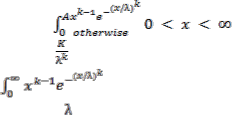
Therefore,
fi(x)=f(x)=
Where A = then
=A dx where k > 0, > 0
The vendor negotiates with an individual customer say Ci, and a compromise is arrived at, to adopt individual JELS ![]() with a price adjustment in the form of discount . This will be generalized to all the values of i (i = 1, 2, 3, . . . n). Then a common strategy for individual lot size and price adjustment has to be designed by the vendor.
with a price adjustment in the form of discount . This will be generalized to all the values of i (i = 1, 2, 3, . . . n). Then a common strategy for individual lot size and price adjustment has to be designed by the vendor.
Corresponding to the optimum value for vendor, customers, the following results can be obtained.![]()
![]()
= [![]() ] where
] where![]()
1(Z) = ![]() dx (2.2.1)
dx (2.2.1)![]()
![]()
= [![]() ] (2.2.2)
] (2.2.2) ![]() (
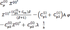
(![]() ) = [
) = [![]() .(
.(![]() )! ─ (
)! ─ (![]() +
+![]() )
)![]()
![]()
A 2(![]() )] where 2(Z) =
)] where 2(Z) = ![]()
![]() dx
dx
(2.2.3)![]()
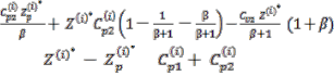
![]() ( ) = [Cv2
( ) = [Cv2![]() ─ (Cv1 + Cv2)
─ (Cv1 + Cv2)
![]()
![]()
A 2( )] (2.2.4)
IJSER © 2012 http://www.ijser.org
International Journal of Scientific & Engineering Research Volume 3, Issue 8, August -2012 5
ISSN 2229-5518
![]() (
(![]() ) =
) =![]()
![]()
![]()
[![]() ─ (
─ (![]() +
+![]() )A
)A![]() 2 (
2 (![]() ) ─
) ─ ![]() +
+ ![]() .(
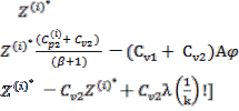
.(![]() )!)] (2.2.5) Cv( ) = [
)!)] (2.2.5) Cv( ) = [![]() ─ (Cv1+Cv2)A 2( )
─ (Cv1+Cv2)A 2( )
─ Cv2![]() + Cv2
+ Cv2 ![]() .(
.(![]() )!] (2.2.6)
)!] (2.2.6)
![]()
![]()
![]()
= [![]() ] (2.2.7)
] (2.2.7) ![]() (
(![]() )= [
)= [![]() 2( )
2( ) ![]() .(
.(![]() )!] (2.2.8) Cv(
)!] (2.2.8) Cv(![]() )=
)=![]()
![]()
![]() 2( )
2( ) ![]() (2.2.9)
(2.2.9)
(a). ![]() <
< ![]() (2.2.10a)
(2.2.10a)
(b). ![]()
![]() >
> ![]() (2.2.10b)
(2.2.10b)
(c). ![]()
![]() =
= ![]() (2.2.10c)
(2.2.10c)
The negotiation between the vendor and the individual customer Ci will be exactly the same as one vendor one customer situation. If the ELS of the vendor be in effect and all the customers change over to respective
JELS, then this will give rise to a situation in which customers will suggest the vendor for a unit price increase. We ignore this because such type of bargain is against the current practice . Hence ignoring such a possibility we concentrate upon the ELS of individual customer in effect trying to switch over to the individual JELS ![]() .
.
If
(i). Cv( ) Cv( ) > 0 (ii). Cp( ) Cp( ) > 0
(![]() )
)
Let both the vendor and the ith customer
adopt JELS , when ith customer’s lot
size This adoption will be done separately for individual customers.
That is each Ci will adopt joint lot size
when
, by this type of adoption the vendor will be at an advantageous position and the ith customer will be at a loss i = 1, 2, 3, . . . n. Now we calculate the difference between the
absolute cost advantage of the vendor and the absolute cost penalty of the ith customer. As,
ACAv (![]() )> ACPp (
)> ACPp (![]() ) Hence,
) Hence,
JACAv( )=ACAv ![]() )
) ![]() ACAp( ) > 0
ACAp( ) > 0
Now ACAv( ) = Cv(![]() )
) ![]()
![]()
![]()
Cv( ) from (2.2.6) & (2.2.9)
IJSER © 2012 http://www.ijser.org
International Journal of Scientific & Engineering Research Volume 3, Issue 8, August -2012 6
ISSN 2229-5518
![]()
![]()
![]()
= [ (Cv1 + Cv2)A![]() 2( Cv2
2( Cv2
+Cv2![]() )!]
)!]![]()
![]() 2(
2(![]() )
)![]()
![]()
![]()
![]()
![]()
![]()
= ![]() (Cv1 + Cv2) 2( ) Cv2
(Cv1 + Cv2) 2( ) Cv2![]() + Cv2
+ Cv2![]()
![]() +
+
(Cv1 + Cv2)![]() 2
2![]() + Cv2
+ Cv2![]()
![]()
Cv2![]() ] (2.3.1)
] (2.3.1)
And
ACAci(![]() )=
)=![]()
![]()
![]()
![]()
=[![]()
![]() A 2( )
A 2( ) ![]() +
+ ![]() ] [
] [![]() ]
]![]()
![]()
![]()
![]()
= [![]()
![]() A 2( )
A 2( ) ![]() +
+ ![]()
![]() +
+![]()
( A 2( )]![]()
![]()
= [ A![]() 2(
2(![]() )
)
- ![]() ] (2.3. 2)
] (2.3. 2)
Therefore, JACA(![]() ) =
) =
ACAv(![]() )
) ![]() ACPp(
ACPp(![]() )
)
= [![]() (Cv1 + Cv2) A(
(Cv1 + Cv2) A(![]() -
- ![]() ) + Cv2(
) + Cv2(![]() )]
)]![]()
= [![]()
![]() A 2(
A 2(![]() )
) ![]() ]
]
= [![]()
![]() + (Cv1 +Cv2) A(
+ (Cv1 +Cv2) A(![]() 2
2![]()
![]() 2
2![]() ) + Cv2(
) + Cv2(![]() )
) ![]()
![]()
![]() (
(![]() ) A(
) A(![]() 2(
2(![]() )
) ![]() ) +
) + ![]() ]
]![]()
![]()
= [ ![]()
![]()
![]() +
+![]()
Cv2( )![]()
![]()
( ) A( ) +(Cv1
+Cv2)A(![]() (
(![]() )]
)]
IJSER © 2012 http://www.ijser.org
International Journal of Scientific & Engineering Research Volume 3, Issue 8, August -2012 7
ISSN 2229-5518
=[
+Cv2( )+( ) A(![]() ) + (Cv1 + Cv2)
) + (Cv1 + Cv2)
A(![]() ]
]
=
[![]()
+ (![]() ) A{
) A{![]() }]
}]
= [![]() + (
+ (![]() +
+ ![]() )A{
)A{![]()
![]()
(2.3.4)
So, the optimum value of the unit price discount offered by the vendor to the customer Ci can be expressed as![]()
= ![]()
![]()
= ![]()
= ![]() JACA (
JACA (![]() ) (2.3.5) Where JACA (
) (2.3.5) Where JACA (![]() ) can be
) can be
evaluated by using the formula given in step
(2.3.4).
Now we shall extend the process to all the n customers we divide the n customers into
three categories depending upon the relation between ![]() and
and ![]() .
.
(i) First category : ![]() (i=1, 2, . . . n)
(i=1, 2, . . . n)
say
The customer for which ![]() , will have no difficulty in compromise between the customers and the vendor. Since for we have by (2.2.10c)
, will have no difficulty in compromise between the customers and the vendor. Since for we have by (2.2.10c)
. Hence the vendor will have no objection in fulfilling the optimum
demand of that particular customer because
that is also the estimated optimum lot size of the vendor.
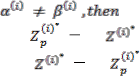
(ii) Second Category : ![]()
![]()
Let for r customers, that is
, for i = m+1, m+2, . . . m+r.
In such a situation the vendor will be at an advantageous position and these m+r customers are bound to incur loss. Hence, the vendor will have to give unit price discounts to the customers Cm+1, Cm+2, . . . Cm+r respectively as follows.![]() JACA(
JACA(![]() ). . . .
). . . . ![]() JACA(
JACA(![]() )
)
Where i = m+1, m+2 . . . m+r
(Since in case of Weibulls distribution E(x)
= ![]() ) Let
) Let
δ = Max ![]() JACA(
JACA(![]() )
)![]()
![]()
for 1 K r (2.3.6)
IJSER © 2012 http://www.ijser.org
International Journal of Scientific & Engineering Research Volume 3, Issue 8, August -2012 8
ISSN 2229-5518
Since δ is the maximum of the unit price discounts mentioned in (2.3.6), therefore the vendor can satisfy all the customers Cm+1, Cm+2, . . Cm+r with this discount and make them agree to adopt their respective individual JELS instead of their original ELS.
(iii). Third Category : ![]()
Let ![]() for rest of the customers, that is for I = (m+r)+1, . . . n.
for rest of the customers, that is for I = (m+r)+1, . . . n.![]() <
< ![]() <
< ![]() for i = (m+r)+1, . . . n
for i = (m+r)+1, . . . n
Let m+r = M![]()
![]() <
< ![]() <
< ![]() for i = M+1, M+2, . . n
for i = M+1, M+2, . . n![]()
So, in this case also the vendor is at an advantageous position and the customers are at a disadvantageous position as ![]()
. Hence vendor will give unit price![]()
Let = Max ![]() JACA(
JACA(![]() )
)
where i = M+1, M+2, . . . n
This ![]() is the maximum unit price discount which will satisfy all the customers
is the maximum unit price discount which will satisfy all the customers
Cm+r+1, Cm+r+2, . . . Cn.
Let ![]() = max (δ ,
= max (δ ,![]() )
)
Obviously this unit price discount ![]() will also satisfy the m customers Ci . . . Cm who have
will also satisfy the m customers Ci . . . Cm who have ![]()
Thus all the customers will be
satisfied with this unit price discount given
by the vendor, ultimately making the compromise at individual JELS level a success. The total inventory stock level available with the vendor at the time of supplying the item to all the n customers should be at least![]()
n
discounts to the customers, CM+1, CM+2, . . . ![]() = Cn respectively as follows.
= Cn respectively as follows.![]() JACA(
JACA(![]() ). . . .
). . . .![]()
![]()
JACA( )
z ( i )*
i 1
Multiple Customers | Vendor | |
Cost Equation | ( ) = [ 2( .( )!] | Cv( ) = [ 2 ( ) |
IJSER © 2012 http://www.ijser.org
International Journal of Scientific & Engineering Research Volume 3, Issue 8, August -2012 9
![]()
![]()
ISSN 2229-5518
Economic Lot Size |
|
|
Minimum Total relevant Cost | ( ) = [ .( )! ─ ( + )A ( |
|
Now we illustrate the model through the following numerical example.
Example : Let the scheduling time t be 1 week.![]()
![]()
![]()
![]()
![]()
![]()
![]()
Distribution with the common density
function f(x)![]()
Where f(x) = ![]() , 0< x < ∞
, 0< x < ∞![]()
With k = 2, = 1 so that A = = 2
Let the random lot sizes Xi for each Ci and Y the random lot size of the vendor be independent and identically distributed random variables belonging to Weibull
2 1 2
![]()
![]()
![]()
= [ ]![]()
![]()
= = 0.1![]()
![]()
![]()
( ) = ![]() = 0.125 (2.4.1)
= 0.125 (2.4.1) ![]() = 0.5 (2.4.2) for the customer C1 (α < β)
= 0.5 (2.4.2) for the customer C1 (α < β)![]()
![]()
( ) = = 0.1
![]() = .447213595 (2.4.3)
= .447213595 (2.4.3)
![]()
![]()
= [![]() ]
]![]()
![]()
= 0.115384615
IJSER © 2012 http://www.ijser.org
International Journal of Scientific & Engineering Research Volume 3, Issue 8, August -2012 10
ISSN 2229-5518
![]()
= ![]() = 0.115384615
= 0.115384615 ![]() = 0.480384461 (2.4.4) Here
= 0.480384461 (2.4.4) Here ![]() >
> ![]() >
> ![]() (2.4.5) for C2 (
(2.4.5) for C2 (![]() )
)![]() (
(![]() ) = 0.125
) = 0.125![]()
![]()
![]() = 0.5 (2.4.6) ( ) = 0.125
= 0.5 (2.4.6) ( ) = 0.125
![]()
![]() = 0.125 (2.4.16)
= 0.125 (2.4.16) ![]() = 0.5 (2.4.17) Here,
= 0.5 (2.4.17) Here, ![]() =
=![]()
For the customer C6 (![]() )
) ![]() (
(![]() ) =.083333333
) =.083333333 ![]() (2.4.18)
(2.4.18) ![]() = 0.109375
= 0.109375![]()
= .467707173 (2.4.19)![]()
= 0.5 (2.4.7)![]()
![]()
![]()
![]()
Here, > (2.4.20)
= = (2.4.8)![]()
![]()
for the customer C3 (![]() ) ( ) =
) ( ) = ![]() = 0.15
= 0.15![]() (
(![]() ) = 0.547722557 (2.4.9)
) = 0.547722557 (2.4.9)![]()
![]()
( )=![]() =0.133333333
=0.133333333 ![]() = 0.516397779 (2.4.10)
= 0.516397779 (2.4.10)
Here, ![]() <
<![]() <
< ![]() (2.4.11)
(2.4.11)
for the customer C4 (![]() )
) ![]() (
(![]() ) = 0.104166666
) = 0.104166666
![]() = .456435463 (2.4.12)
= .456435463 (2.4.12)
![]() (
(![]() ) = 0.1171875
) = 0.1171875![]()
![]() = .484122918 (2.4.13) Here,
= .484122918 (2.4.13) Here, ![]() >
>
For the customer C5 (![]()
![]() (
(![]() ) = 0.125 (2.4.14)
) = 0.125 (2.4.14)![]()
= 0.5 (2.4.15)
For the customer C7 (![]() )
) ![]() (
(![]() ) = 0.078125
) = 0.078125
![]() = .395284707 (2.4.21)
= .395284707 (2.4.21)
![]()
![]() (
(![]() ) = 0.104166666
) = 0.104166666![]()
![]() = .456435464 (2.4.22) Here,
= .456435464 (2.4.22) Here, ![]() >
>
For the customer C8 (![]() )
)![]() (
(![]() ) = 0.125 (2.4.23)
) = 0.125 (2.4.23) ![]() = 0.5 (2.4.24)
= 0.5 (2.4.24) ![]() (
(![]() ) = 0.125
) = 0.125![]() = 0.5 (2.4.25) Here,
= 0.5 (2.4.25) Here, ![]() =
=![]()
![]() (2.4.26) Let us find the values C1, C4, C6, C7
(2.4.26) Let us find the values C1, C4, C6, C7![]()
Cv(![]() ) = [
) = [
IJSER © 2012 http://www.ijser.org
International Journal of Scientific & Engineering Research Volume 3, Issue 8, August -2012 11
ISSN 2229-5518
![]()
] = .02268046![]()
![]()
( )=
![]() for customer C1
for customer C1
![]()
(![]() ) =
) = ![]() = 0.029814239 [(
= 0.029814239 [(![]() )!=.760326419 According to sterling function] (2.4.27)
)!=.760326419 According to sterling function] (2.4.27)![]() =17.29479152
=17.29479152![]()
![]()
( ) = ![]() = 0.03695265
= 0.03695265![]()
![]()
=[![]() - ( ) A
- ( ) A![]() +
+ ![]() ]
]
= 17.11010273 (2.4.28) ![]() -
- ![]() > 0
> 0
for customer C4![]()
(![]() ) =
) = ![]() = 0.031696906
= 0.031696906![]()
![]()
![]()
![]() = 17.22714375 (2.4.29) ( ) = = 0.037822102
= 17.22714375 (2.4.29) ( ) = = 0.037822102
![]()
=17.71199903 (2.4.31)![]()
= ![]() = .034103647
= .034103647![]()
![]()
![]()
( )=![]() - ( )
- ( )![]()
A (![]() ) -
) - ![]()
=17.16135386 (2.4.32) ![]() -Cv(
-Cv(![]() )>0
)>0
by (2.4.31) & (2.4.32)
For customer C7![]()
(![]() ) =
) = ![]() =.020587745
=.020587745![]()
![]()
![]()
(![]() )=
)=![]() - ( ) A (
- ( ) A (![]() )
)![]()
- (![]() ) +
) + ![]()
=17.89570776 (2.4.33)![]()
![]()
= = .031696907![]()
![]() (
(![]() )= [
)= [![]()
![]() (
(![]() )= -(
)= -(![]() )
)![]()
![]()
![]()
A ( ) -
]
= 17.09967683 (2.4.30)![]()
![]()
- Cv( ) > 0
=17.22714343 (2.4.34) ![]() -Cv(
-Cv(![]() )>0
)>0
by (2.4.33) & (2.4.34)
for customer C6
IJSER © 2012 http://www.ijser.org
International Journal of Scientific & Engineering Research Volume 3, Issue 8, August -2012 12
ISSN 2229-5518
Let us calculate![]()
ACAv(![]() & AC
& AC![]() (
(
for i = 1,2,3,4,5,6,7,8
ACAv(![]() =
=![]() - Cv(
- Cv(![]() )
)
= 0.18468879 (2.4.35) To calculate ACAc1 (![]() ) , we have to calculate
) , we have to calculate ![]() (
(![]() ) and
) and ![]() (
(![]() )
)![]()
![]()
![]()
( )=[![]() - ( )
- ( )![]()
A (![]() ) –
) – ![]() +
+ ![]() !]
!]
=9.29410441 (2.4.36)![]() (
(![]() ) = [
) = [ ![]() - (
- (![]() ) A
) A![]() )]
)]
=9.24368058 (2.4.37)![]() (
(![]() )-
)- ![]() (
(![]() ) =.05042383 (2.4.38) Hence
) =.05042383 (2.4.38) Hence
ACAv(![]() )> ACPc1(
)> ACPc1(![]() )
)
![]()
JACA( )=0.13426496
C1 = ![]() JACA(
JACA(![]() )
)
=0.088294288 (2.4.41) For customer C4![]()
![]() ( )=[
( )=[![]() - (
- (![]() )
)![]()
A (![]() ) -
) - ![]() +
+ ![]() ]
]
=9.154992091 (2.4.42)![]() (
(![]() ) = [
) = [ ![]() - (
- (![]() ) A
) A![]() )]
)]
= 9.12088486 (2.4.43)
ACP![]() (
(![]() )=
)= ![]()
= .034107231 (2.4.44) ACAv(![]() )=0.12746692 (2.4.45) Hence,
)=0.12746692 (2.4.45) Hence,
![]()
ACAv(![]() ) > ACP
) > ACP![]() (
(![]() ) JACA(
) JACA(![]() )=.093359689 (2.4.46) JACA(
)=.093359689 (2.4.46) JACA(![]() )
)
![]()
=[ +( +![]()
JACA(![]() )
)![]()
=[ +( +
(2.4.39)![]() )(A(
)(A(![]() ))]
))]
=.093197265 (2.4.47) Thus (2.4.46) & (2.4.47) agree with each![]() )(A(
)(A(![]() ))]
))]
=0.13426496 (2.4.40) Thus the results of (2.4.39) & (2.4.40) tally optimum discount to the customer
other
![]() Optimum discount to C4
Optimum discount to C4
=![]() JACA(
JACA(![]() )
)
= .035430171 (2.4.48) For customer C6
IJSER © 2012 http://www.ijser.org
International Journal of Scientific & Engineering Research Volume 3, Issue 8, August -2012 13
ISSN 2229-5518
![]()
![]()
![]()
= [ - ( )![]()
A (![]() ) -
) - ![]() +
+ ![]() ]
]
=7.955858345 (2.4.49)
![]() =[
=[![]() -(
-(![]() ) A
) A![]() (
(![]() )]
)]
=7.810574384 (2.4.50)
ACP![]() (
(![]() )=
)= ![]()
= 0.145283961 (2.4.51)
ACAv(![]() )=0.55064517 (2.4.52) Hence ,
)=0.55064517 (2.4.52) Hence ,
ACAv(![]() ) >ACP
) >ACP![]() (
(![]() ) JACA(
) JACA(![]() )=.405361209 (2.4.53) By formula, JACA(
)=.405361209 (2.4.53) By formula, JACA(![]() )
)![]()
![]()
=[![]() +( + )
+( + )
(A(![]() ))]
))]
=0.40536121 (2.4.54) Thus, (2.4.53) & (2.4.54) tally with each other.
![]() Optimum discount to
Optimum discount to
C6 = ![]() JACA (
JACA (![]() )
)
= .266570515 (2.4.55) For customer C7![]()
![]()
![]()
= [ - ( )![]()
A (![]() ) -
) - ![]() +
+ ![]() ]
]
= 10.13502328 (2.4.56)
![]() -(
-(![]() )
)
A![]() (
(![]() )]
)]
= 9.93606566 (2.4.57) ACP![]() (
(![]() )=
)= ![]()
= 0.19895762 (2.4.58)
ACAv(![]() )=0.66856433 (2.4.59)
)=0.66856433 (2.4.59)
Hence,![]()
ACAv(![]() ) >ACP JACA(
) >ACP JACA(![]() )=0.46960671 (2.4.60) Again by formula , JACA(
)=0.46960671 (2.4.60) Again by formula , JACA(![]() )
)
![]()
= [![]() + ( +
+ ( + ![]() )A{(
)A{(![]() )}]
)}]
=0.469606707 (2.4.61)
Thus the result (2.4.60) is in agreement with the result (2.4.61)
![]() for customer C7
for customer C7
Optimum discount= ![]() JACA (
JACA (![]() )
)
=0.308819143 (2.4.62)![]()
=max{0.088294288,.035430171, .266570515,
IJSER © 2012 http://www.ijser.org
International Journal of Scientific & Engineering Research Volume 3, Issue 8, August -2012 14
ISSN 2229-5518
0.308819143}
=0.308819143 (2.4.63) Third Category : ![]()
![]() is the only member belonging to this
is the only member belonging to this
category for the customer ![]()
![]()
![]() (
(![]() = [
= [
]![]() =
=![]() = 0.054772255
= 0.054772255![]()
![]()
( ) = ![]() = 0.045902024
= 0.045902024 ![]() (
(![]() =17.26771562 (2.4.64)
=17.26771562 (2.4.64)![]()
![]()
![]()
( )=[![]() -( )
-( )![]()
A (![]() ) -
) - ![]() ]
]![]()
=17.10146982 (2.4.65) ACAv(![]() )=0.1662458 (2.4.66)
)=0.1662458 (2.4.66) ![]() = [
= [![]() - (
- (![]() )
)
A (![]() ) -
) - ![]() +
+ ![]() ]
]
=9.526449472 (2.4.67)![]() (
(![]() ) = [
) = [ ![]() - (
- (![]() ) A
) A![]() )]
)]
= 9.484273256 (2.4.68)
ACP![]() (
(![]() )=
)= ![]()
= 0.042176216 (2.4.69)
Hence,
ACAv(![]() )>ACP
)>ACP![]() (
(![]() )
) ![]() JACA(
JACA(![]() )=0.124069584
)=0.124069584
(2.4.70)
By formula
JACA(![]() )
)![]()
![]()
=[![]() +( + ) (A(
+( + ) (A(![]()
![]() ))]
))]
= 0.12406958 (2.4.71) Thus the result (2.4.70) is agreement with (2.4.71)
Therefore the optimum value of discount offered to ![]()
= ![]() JACA (
JACA (![]() )
)
= 0.081589681 (2..4.72)
As ![]() is the only customer belonging to third category
is the only customer belonging to third category![]()
![]() =0.081589681 (2.4.73) From (2.4.72) & (2.4.73) the optimum value of the uniform discount given to all the eight customers is given by
=0.081589681 (2.4.73) From (2.4.72) & (2.4.73) the optimum value of the uniform discount given to all the eight customers is given by
( )=max(0.308819143, 0.0815896801)
=0.308819143 (2.4.74)
IJSER © 2012 http://www.ijser.org
International Journal of Scientific & Engineering Research Volume 3, Issue 8, August -2012 15
ISSN 2229-5518
The total inventory stock level available with the vendor at the time of supplying the item to all the eight customers should be at least![]()
= ![]()
![]()
=
=3.905047795 (2.4.75)
In this paper, the buyer-vendor area of the supply chain management problem discussed. Here mainly focused on the Joint Economic Lot Size for the buyer and vendor model. There are many models which recently extended Banerjee's JELS. Banerjee's (1986), showed that his model worked for a single product, single buyer and single vendor. He showed great savings with his model. Here a model developed for Single vendor and multiple buyer situations using Weibulls Distribution.
In this model a detailed analysis has
been made to show how inventory related costs vary through closer interaction between the vendor and the customer. The unit price and the order quantity etc. are settled by negotiation between both the parties to minimize the total relevant costs. If JELS is adopted by both, the gain or loss are to be shared reasonably between them so that both will come to a mutual compromise. JELS model not only minimize the total relevant cost of the system but also searches a common lot size with no loss to both. In this model the set up cost is assumed to be zero. The effect of this JELS model can be verified in various other situation with demand satisfying different continuous probability distributions. The demand of the customer and stock level of the vendor are non-negative quantities.
[1] Monahan, J. P. (1984), A Quantity Discount Pricing Model to Increase Vendor Profits, Management Science 30, 720-726.
[2] Lee, H. L. and Rosenblatt, M. J. (1986), A Generalized Quantity Discount Pricing Model to Increase Suppliers Profits, Management Science, 32 1177-1185
[3] Banerjee A. (1986 a), A Joint Economic Lot size Model for purchaser and vendor, Decision science 17, 292-311.
[4] Jogelkar, P. N. (1988), Comments on A Quantity Discount pricing Model to Increase Vendor Profits, Management Science 31,
1391-1398.
[5] Goyal, S.K. (1988), A joint economic lot size model for purchaser and vendor: a comment. Decision Sciences, 19, 236-241.
[6] Goyal, S. K and Gupta, Y. P. (1989), Integrated Inventory Models: the Buyer- vendor co-ordination, European Journal of operations research 41, 261-269.
[7] Vishwanathan S. (1998), Optimal strategy for the integrated vendor-buyer inventory model. European Journal of Operational Research; 105: 38-42.
[8] Chatterjee, A. K., Ravi, R. (1991), Joint Economic Lot Size model with delivery in Sub-batches OPSEARCH, 28, 119-124.
[9] Agrawal, A. K., Raju D. A. (1996), Improved Joint Economic Lot Size model for a purchaser and a vendor. Department of
IJSER © 2012 http://www.ijser.org
International Journal of Scientific & Engineering Research Volume 3, Issue 8, August -2012 16
ISSN 2229-5518
Mechanical Engineering, Institute of Technology, Benras Hindu University, Varanasi, India.
[10] Thomas, D. J., Griffin, D. J. (1996). Coordinated supply chain management. European Journal of Operational Research,
94, 1-15.
[11] Narasimhan and Carter (1998), Integrating environmental management and supply chain strategies, Volume: 14, Wiley InterScience, Pages: 1-19.
[12] Affisco J.F. , Paknejad M.J., and Nasri F., (2002), Quality improvement and setup reproduction in the Joint Economic Lot Size model. European Journal of Operations Research , 142, 497-508.
[13] Pourakbar, M., Farahani, Z.R. & Asgari, N. (2007), A Joint Economic Lot Size model for an Integrated Supply network using genetic algorithm. Applied Mathematics and Computation , 189(1). 583-
596.
[14] Ben-Daya M., Darwish M. and Ertogral K.,( 2008), The Joint Economic Lot Sizing problem. A review and extensions. European Journal of Operational Research, 185/2, 726-
742.
[15] Pan J.C.-H & Yang M. –F.(2008), Integrated inventory models with fuzzy annual demand and fuzzy production rate in a Supply Chain. International Journal of
Production Research 46(3), 753-770.
IJSER © 2012 http://www.ijser.org