International Journal of Scientific & Engineering Research, Volume 3, Issue 7, July-2012 1
ISSN 2229-5518
A Comparitive Study Of Kalman Filter, Extended Kalman Filter And Unscented Kalman Filter For Harmonic Analysis Of The Non-Stationary Signals
A.UmaMageswari, J.Joseph Ignatious ,R.Vinodha.
Abstract –– The accurate measurement of harmonic level is essential for designing harmonic filters and monitoring the stress to which the communication devices are subjected due to harmonics and specifying digital filtering techniques for phasor measurements . This paper presents an integrated approach to design an optimal estimator for the measurement of frequency and harmonic components of a time varying signal embedded in low signal-to noise ratio. This led to the study of Kalman, Extended Kalman and Unscented Kalman filter characteristics and a subsequent implementation of the study to design these filters. W e have employed the Extended Kalman filter and Unscented Kalman filter algorithms to estimate the voltage magnitude in the presence of random noise and distortions. Kalman filter being an optimal estimator to track the signal corrupted with noise and harmonic distortion quite accurately. Tracking of harmonic components of a dynamic signal in communication system can easily be done using EKF and UKF algorithms and their results are compared.
Keywords— Kalman filter, extended Kalman filter, Unscented Kalman filter, Unscented transformation, Harmonic A nalysis, Non-stationary signals,guassian random variable.
—————————— ——————————
The problem of estimating frequency and other parameters of sinusoidal signal in white noise in radar, nuclear magnetic resonance, power network etc, have been extensively studied. Among the several methods for frequency, amplitude and phase estimation of non-stationary signals, Discrete Fourier Transform (DFT) and Fast Fourier Transform (FFT) are widely used. However both the above methods suffer from aliasing ,leakage and picket fence effects and hence need error compensation and adaptive window width .Some of the known signal processing techniques like artificial neural networks ,linear prediction technique adaptive filter, supervised Gauss-Newton algorithm ,least- error square and its variants, extended Kalman filters, have been used for time-varying signal parameter estimation. Most of these algorithms require heavy computational outlay and suffer from inaccuracies in the presence of noise with low signal to noise ratio (SNR).![]()
![]() J.Joseph Ignatious, Research Scholar,
J.Joseph Ignatious, Research Scholar,
Faculty of Engineering, Annamalai University, Chidambaram,TamilNadu,India.
![]() A.UmaMageswary, Research Scholar,
A.UmaMageswary, Research Scholar,
Faculty of Engineering, Annamalai University,
Chidambaram,TamilNadu,India.
E-mail: uma.sathya123@yahoo.co.in
![]() R.Vinodha, Associate Professor, Dept of E & I, Faculty of Engineering, Annamalai University,
R.Vinodha, Associate Professor, Dept of E & I, Faculty of Engineering, Annamalai University,
Chidambaram,TamilNadu,India.
Almost all the real time functions are non-linear and all the systems can be represented as discrete time system to a great extent of accuracy using very small time steps. Now the problem is to estimate the states of this discrete-time controlled process and the process is generally expressed with the help of linear stochastic difference equation. This estimation can be easily and accurately done by the Kalman Filter.
But when the process and the measurement system are non-linear EKF and UKF are implemented. A KF that linearizes about the current mean and covariance using any linearizing function is called EKF. In this the partial derivatives of the process as well as measurement functions are used to compute estimates in the presence of non-linear function.
In this paper, section2 deals with the kalman filter algorithm , section 3 deals with the Extended kalman filter algorithm, section 4 deals with the unscented kalman filter, section 5 deals about the comparison of KF,EKF,UKF estimation approaches and section 6 deals about the estimation of harmonics using EKF,UKF methodology and simulation results and section 7 deals about conclusion.
It is the Optimal solution for linear-Gaussian case.
IJSER © 2012
International Journal of Scientific & Engineering Research, Volume 3, Issue 7, July-2012 2
ISSN 2229-5518
Now we are going to made an Assumptions are State model is known linear function of last state and Gaussian noise signal, Sensory model is known linear function of state and Gaussian noise signal and Posterior density function is Gaussian. It’s Used to provide the closed form recursive solution of estimation of linear discrete time dynamic systems
State model is considered as linear model and expressed as
noise, the covariance of the observation noise; and sometimes the control-input model for each time-step k , Fk, Hk , Qk, Rk, Bk, respectively as described further.
The KF model assumes the state at (k − 1) helps in measuring the true state at time k .![]()
XK=AK-1 XK-1+qK-1
YK=HK XK+rk
Kalman Filter Uses linear transformation and has following steps are Prediction step-next state of the system is predicted for previous measurement and Update step-current state of the system estimated from the measurement at the step.
The Kalman Filter is an algorithm to generate estimates of the true and calculated values, first by predicting a value, then calculating the uncertainty of the above value and finding an weighted average of both the predicted and measured values. Most weight is given to the value with least uncertainity. The result obtained by this method gives estimates more closer to true values.
The Kalman Filter estimates a process by using a feedback control like form. The operation can be described as the process is estimated by the filter at some point of time and the feedback is obtained in the form of noisy measurements. The Kalman filter equations can be divided into two categories: time update equations and measurement update equations. To obtain the a priori estimates for the next time step the time update equations project forward (in time) the current state and error covariance estimates. The measurement update equations get the feedback to obtain an improved a posteriori estimate incorpoating a new measurement into the a priori estimate.
KF is based on linear and non-linear dynamical systems discretized in the time domain. A vector of real numbers represents the state of the system. At each discrete time increment, a new state is generated applying a linear operator, with some noise added. Then, the observed states are generated using another linear operator with some added noise usually called as the measurement noise.
To use the KF to get estimations of the internal states of a process where only a sequence of noisy observations are known as inputs, the process is modelled in accordance with the state space representation of the Kalman filter. It means specifying the following matrices: the state- transition model, the observation model, the covariance of the process
Where
Fk is the state transition state space model and it is applied to the previous state xk−1;
Bk is the control-input state space model and it is
applied to the control vector uk;
Wk being t h e process noise and is d r a w n from a multivariate normal distribution with zero
mean and covariance Qk.![]()
An observation zk of the true state xk time k is made according to![]()
Here Hk is the observation state space model which helps in mapping the observed space from true space and vk is the observation or measurement noise (Gaussian white noise) with zero mean and covariance Rk.![]()
Starting from the initial states to the noise vectors at each step are mutually independent.
As we know the real systems that are inspiration for all these estimators like Kalman Filter are governed by non- linear functions. So we always need the advanced version of the Filters that are basically designed for linear filters. Similarly it is said that in estimation theory, the extended Kalman filter (EKF) is the nonlinear version of the Kalman filter. This non-linear filter linearizes about the current mean and covariance. At one time, the EKF might have been considered the standard in the theory of nonlinear state estimation navigation systems and GPS. However, as described below, with the introduction of the Unscented Kalman filter (UKF), the EKF might not enjoy the status of being the standard filter as the UKF is more robust and more accurate in its estimation of error.
IJSER © 2012
International Journal of Scientific & Engineering Research, Volume 3, Issue 7, July-2012 3
ISSN 2229-5518
In the EKF, the state transition and observation state space models may not be linear functions of the state but might be many non-linear functions.![]()
![]()
Where wk and vk are the process and observation noises which are both assumed to be zero mean multivariate Gaussian noise with covariance Qk and Rk respectively.The functions f a n d h use the previous estimate and help in computing the predicted state and again the predicted state is used to calculate the predicted measurement. However, f and h cannot be used to the covariance directly. So a matrix of partial derivatives (the Jacobian) c o m p u t a t i o n is required.At each time step with the help of current predicted states the Jacobian is calculated. These matrices are used in the KF equations. This process actually linearizes the non- linear function around the present estimate.
Predicted state![]()
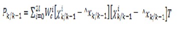
Predicted estimate covariance![]()
Innovation or measurement residual![]()
Innovation (or residual) covariance![]()
Optimal Kalman gain![]()
Updated state estimate![]()
![]()
Updated estimate covariance
Where the state transition and observation matrices are defined to be the following Jacobians![]()
![]()
The key to using an EKF is to be able to represent the system with a mathematical model. That is, the EKF designer needs to understand the system well enough to be able to describe its behaviour with differential equation. In practice, this is often the most difficult part of implementing a Kalman filter. Another challenge in Kalman filtering is to be able to accurately model the noise in the system.
In the presence of non-linear functions the predicted states are approximated as the function of prior mean. The covariances are determined by linearizing the dynamic equations![]()
a n d t h e n t h e p o s t e r i o r c o v a r i a n c e m a t r i c e s a r e determined analytically for the linear system in EKF approach. In case of the EKF, a GRV is determined approximating the state distribution and then this GRV is propagated analytically through the ``first-order'' linearization of the nonlinear system. In this case the EKF can be credited with providing ``first-order'' approximations to the optimal terms such as optimal prediction, optimal gain. But these approximations are not helpful always. Where the non- linearity value is more it can even introduce large errors in the true posterior mean as well as in the covariance of the transformed (Gaussian) random variable. This is not being a healthy approach to linearization might lead to sub-optimal performance and sometimes divergence (instability) of the filter. It is these ``flaws'' which will be amended in the next section using the UKF.
When the state transition and observation state space models – the predict and update functions f and h are
highly non-linear, the EKF cannot give up to the mark performance because the linearization of the underlying non-linear model propagates the covariance. Although EKF is straightforward and simple it suffers from instability due to linearization and erroneous parameters, costly calculation of Jacobean matrices, and the biased nature of its estimates. The UKF is considered in this paper to overcome the disadvantages of EKF.The UKF belongs to the family of sigma-point filters and uses an unscented transformation that computes the statistics of a random variable undergoing
IJSER © 2012
International Journal of Scientific & Engineering Research, Volume 3, Issue 7, July-2012 4
ISSN 2229-5518
nonlinear transformation.The main advantage of UKF is that it does not use linearization for calculating the state predictions, covariance matrices and thus it provides accurate Kalman gain estimates. Instead of linearizing the Jacobean matrices, the UKF uses a deterministic sampling approach to capture mean and covariance estimates with a minimal set of
2 L + 1, sigma points (L is the state dimension) based on a
square-root decomposition of the prior covariance. These
sigma points are propagated through the nonlinearity, without approximation, and a weighted mean and covariance is found. Like the EKF, the UKF uses a recursive algorithm that uses the system model, measurements, and known statistics of the noise mixed with the signal. The UKF was originally designed to estimate the states of a dynamic system and for nonlinear control applications.
The UKF update can be used independently in the UKF prediction in co-ordination with a linear update. The mean and covariance of the process noise is used in increasing the estimated state and covariance.![]()
![]()
The augmented state and covariance assist in derivation of a set of 2L+1 sigma points and L is the
method is numerically efficient and stable.The transition function f helps in propagating the sigma points.![]()
The predicted state and covariance are produced by recombination of the weighted sigma points.![]()
And the weights for the state and covariance are given by:![]()
![]()
![]()
Αa and κ control the spread of the sigma points. β is related to
− 3
dimension of the augmented state.
the distribution of x. Normal values Are α = 10
, κ = 0 and β![]()
![]()
![]()
![]()
And![]()
Is the ith column of the matrix square root of![]()
The Cholesky decomposition method should be used for the calculation of matrix square root.Because this
= 2. If the true distribution of x is Gaussian, β = 2 is
optimal.The same augmentation of the predicted state
and covariance is done with the mean and Covariance of the measurement noise.
The most general form of state space model is the non-linear model. The models are basically consist of two function f and h which govern the state propagation and measurements respectively. w and v are the process and measurement noises respectively, u is the process input and k is the discrete time.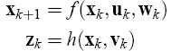
This is the actual model where as the linear state- space model is the model where the functions f and h are both linear in state and input. The function then can be expressed using matrices F, B and H, reducing state
IJSER © 2012
International Journal of Scientific & Engineering Research, Volume 3, Issue 7, July-2012 5
ISSN 2229-5518
propagations to linear algebra casing easier calculation and analysis. The model equations can be written as: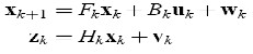
Certain constraints on the process model can make the estimation problem easier. The constraints in case of Kalman filter are both the functions f and h are to be linear, noise terms w and v uncorrelated, Gaussian and white with zero mean. The model being linear and input being Gaussian we have the knowledge that the output will also be Gaussian. The state and output pdf will therefore always be normally distributed and the knowledge of mean and covariance will suffice .Estimation using Kalman filter is easier as it incorporates almost all linear calculation except a matrix inversion
Almost all real life process is non-linear and needed to be linearized before they can be estimated by means of a KF. By calculating the Jacobian of f and h around the estimated state, this problem of non-linearity is solved by EKF. The calculation of Jacobian yields a trajectory of the model function centered around the state.
Fig-1. EKF linearizing a non-linear function around the mean of a Gaussian distribution
Propagation of GRV through non-linear functions cause trouble many times and by applying a new technique called the unscented transform it can be solved. Ins tead of linearizing a non- linear function it uses 2N+1 sigma points for N states and then propagates these points through the actual non-linear function, eliminating linearization altogether. The points are chosen such that their mean, covariance as well as other higher order moments also match the GVR. These propagated points help in recalculating the mean and covariance yielding more accurate results compared to ordinary function linearization.
The underlying idea is to approximate the probability distribution instead of the function. This strategy helps in decrement in computational complexities at the same time increasing estimation accuracy, gaining faster and more accurate results.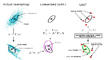
Fig-2. Example of mean and covariance propagation
The unscented transform approach provides another advantage of t r e a t i n g noise in a nonlinear fashion to account for non-Gaussian or non-additive noises. For doing so firstly noise is propagated through the functions by first augmenting the state vector including the noise sources. This technique was first introduced by Julier and later developed by Merwe. Sigma point samples are then selected from the augmented state xa, which includes the noise values. This technique results in the accuracy of process and measurement noise capture with same accuracy as that of the state, which in turn increases the accuracy for non-additive noise sources.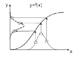
Fig-4. UKF propagating sigma points from a Gaussian distribution through a non-linear function
IJSER © 2012
International Journal of Scientific & Engineering Research, Volume 3, Issue 7, July-2012 6
ISSN 2229-5518
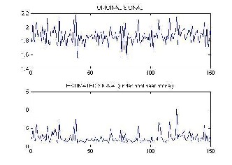
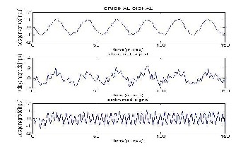
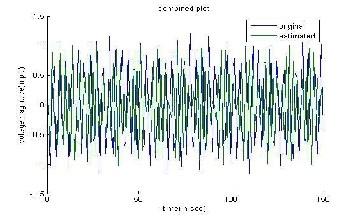
Firstly a static signal as given below is modelled with the help of EKF and UKF algorithms.The test signals with these non-linearities and the Gaussian noise is used as the process and estimation of the amplitude is carried out with the help of EKF and UKF methods. The estimated and the original signal and a comparison between them are given in the following section. In case of EKF the mean square error is calculated for the estimated signal.
Xk=(sinxk)+exp(xk)+wk
Consider a signal consisting of M sinusoids which can be modelled as given below.![]()
Where Aik, wi, Фi, tk and vk a r e amplitude, frequency and phase of the i- th sinusoid respectively and tk
(a)
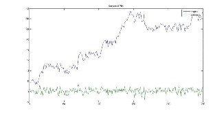
Fig- 5(a) Extended Kalman Filter Output
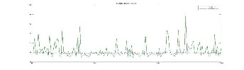
(b) Mean Square Error in Extended Kalman Filter
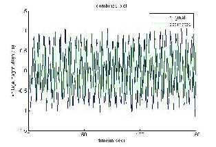
(c) Unscented Kalman Filter Output estimation
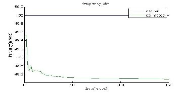
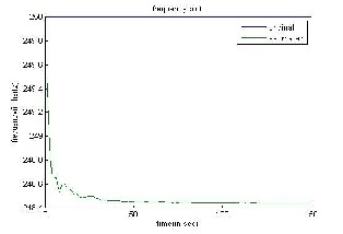
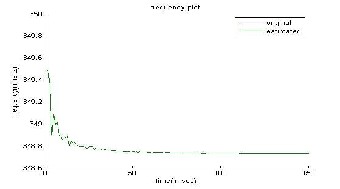
(d) Fundamental Amplitude And Frequency Estimation using Ukf
(e) Fundamental amplitude and frequency estimation using UKF
rd
is the k-th sample of the sampling time and vk is a zero mean
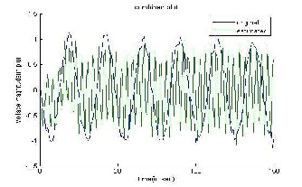
( f) 3
Harmonic amplitude estimation using UKF
Gaussian white noise.
th
(g) 5 Harmonic amplitude and frequenc y estimation using UKF
th
In this paper a signal like this has been used but keeping o
(h) 7
th
(i) 7
Harmonic Aplitude Estimation (Ukf)
Harmonic amplitude and frequenc y estimation using UKF
amplitude 1p.u. and frequency 50Hz and phases 0
and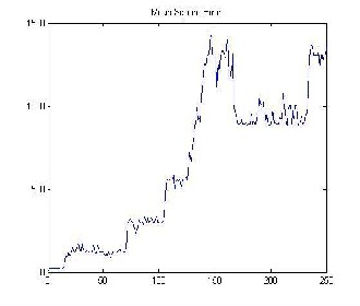
generating process and measurement noises with the help of random number generator. The amplitude and frequency estimation has been done of the signal starting from
th
, th and 7
harmonic
signal. Both the original and estimated voltage amplitude value and frequency values have been compared.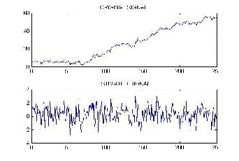
IJSER © 2012
(b)
International Journal of Scientific & Engineering Research, Volume 3, Issue 7, July-2012 7
ISSN 2229-5518
 (e)
(e)
(c) 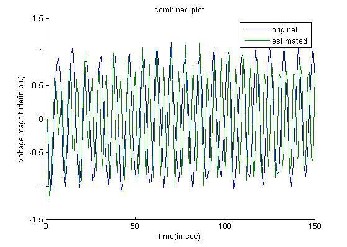
(d) 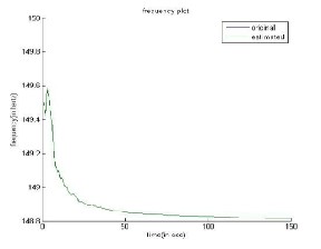
 (f)
(f)
IJSER © 2012
International Journal of Scientific & Engineering Research, Volume 3, Issue 7, July-2012 8
ISSN 2229-5518
(g)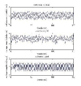
(h)
(i)
First we briefly introduce the concept of discrete-time state space models. After that we consider linear, discrete-time state space models in more detail and review Kalman filter, which is the basic method for recursively solving the linear state space estimation problems. After that the function of Kalman filter its usage in this toolbox in demonstrated with one example (CWPA-model).Next we move from linear to nonlinear state space models and review the extended Kalman filter, which is the classical extension to Kalman filter for nonlinear estimation.
The usage of EKF in this toolbox is illustrated exclusively with one example (Tracking a random sine signal), which also compares the performances of KF, EKF and UKF. After EKF we review unscented Kalman filter, which is a extension to traditional Kalman filter to cover nonlinear filtering problems.
The problem of estimating frequency and amplitude parameters of sinusoidal signal in white noise in radar, nuclear magnetic resonance,
IJSER © 2012
International Journal of Scientific & Engineering Research, Volume 3, Issue 7, July-2012 9
ISSN 2229-5518
power networks etc., h a v e been extensively studied. By comparing KF, EKF & UKF , the main advantages of the unscented transformation used in UKF is that it does not use linearization for computing the state and error covariance matrices resulting in a more accurate estimation of the parameters of a nonstationary signal. However its accuracy significantly reduces if the SNR is low and the noise covariance and some of the parameters used in the unscented transformation are not chosen correctly.Therefore considering the above drawback of EKF, it is proposed to use adaptive particle swarm optimization technique in best signal tracking performance ,it is found to be superior to the conventional particle swarm optimization (PSO) for the optimal choice of UKF parameter and error covariances. This results in better local and global searching ability of the particle which in turn improves the convergence of the velocity and better accuracy of the unscented Kalman filter.
[1] A.Routray, A.K.Pradhan, K.P.Rao, A novel Kalman filter for frequency estimation of distorted signal in power systems,IEEE transaction on instrumentation and measurement-2002.
[2] D.W .P.Thomas, M.S.W oolfson, Evaluation of frequency tracking methods, IEEE Transaction on power delivery-2001.
[3] H.C. So, K.W . Chan, Y.T. Chan, K.C. Ho, Linear prediction approach forefficient frequency estimation of multiple real sinusoids: algorithm and analysis, IEEE Transactions on Signal Processing - 2005
[4] J.Z.Yang, C.S.Yu, C.W .Liu, A new method for power signal harmonic analysis, IEEE transaction on power delivery-2005.
[5] P.K.Dash,.D.P.Swain,A.C liew,An adaptive linear combiner for on line tracking of power system harmonics, IEEE Transaction on power delivery-1996.
[6] P.K.Dash, Shazia Hasan, B.K.Panigrahi, Hybrid UKF and PSO Technique for Non stationary signals, Elsevier-2003.
[7] S.J.JULIER, J.K.UHLMANN, Unscented filtering and nonlinear estimation, Proceedings of the IEEE-2000
[8] S.J. Julier, J.K. Uhlmann, Unscented filtering and nonlinear estimation, Proceedings of the IEEE 92 -2004
[9] S. Julier, J. Uhlmann, H.F. Durrant-W hyte, A new method for the nonlinear transformation of means and covariances in filters and estimators, IEEE Transactions on Automatic Control -2008
[10] Y.N. wang, J.C. Gu, C.M. Cheu, An improved adaline algorithm for online tracking of harmonic components International Journal of
Power and Energy Systems -2003
IJSER © 2012