International Journal of Scientific & Engineering Research, Volume 5, Issue 9, September-2014 5
ISSN 2229-5518
Vision based Quality Monitoring and Control
Using Adaptive Threshold Technique
Karim M. Taha, M. A. Metwally, F. M. Ahmed, G. El-Nashar
Abstract In this paper, a real time quality monitoring and control in multicolor printing is proposed using online mechatronic system based on computer vision. Theoretical and practical study for automatic detection of register marks through an adaptive threshold value selection algorithm. The proposed system provides an automatic control of the press machine to be able to quantify and compensate the miss- registration happens in printing setup or during operation. The proposed mechatronic system uses a CMOS image sensor to capture the printed register mark image data in real time. Further image processing and analyzing is carried out under MATLAB environment. The color segmentation algorithm involves an adaptive threshold value selection technique to enhance the overall system performance. The geometrical color to color deviation is compensated through DC motor controlled by the decision making algorithm. The system was applied to a pen plotter as a simulation of press machine and succeeded to achieve the required task.
Index Terms Algorithms, Color segmentation, Computer vision, Image processing, Mechatronics, Quality control.
—————————— ——————————
RINTING quality control is often an extensive target of business for professional press houses. High quality multicolor printing often relies on many factors including ink, paper, and environ-
mental conditions. In multicolor printing machines, the exact superimpo- sition of overprinting different color separations for cyan, magenta, yel-
low, and black is essential for a good quality multicolor printing. The operator must check the color registration marks with an accuracy of approximately 1/100 mm in circumferential and lateral direction. In or- der to check the printed sheet while the printing process is running, the operator must drag a sheet from the delivery pile and inspect the printing defects to take the action required to correct these defects. This often leads to considerable amount of wasted time and materials. Also, it af- fects the printing quality [1]. So, a low cost automated process is re- quired to overcome the mentioned disadvantages and to improve the printing quality.
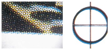
In color printing, registration is the method of correlating overlapping colors on one single image. There are many different styles and types of registration, many of which employ the alignment of specific marks [2] (see Figure 1).
Fig 1: Color register deviation
The miss-registration term is defined as the geometrically difference between each individual color separation being printed on the paper substrate (see Figure 2). The observer can notice the shift in magenta print slightly to the left and the shift in cyan color print slightly to the right.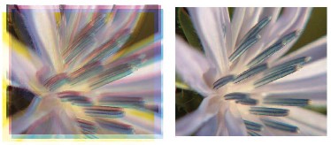
Fig 2: Registration misalignment example
The quality monitoring process of a product can be carried out with a variety of methods and techniques. However, this product can be any kind of industrial products including the print media products. Recently,
computer vision technique is one of the most common techniques being used to monitor the quality of a certain product [3].
The block diagram (see Figure 3) illustrates the overall work flow of the proposed mechatronic system.
Fig 3: The workflow of the proposed mechatronic system
IJSER © 2014 http://www.ijser.org
International Journal of Scientific & Engineering Research, Volume 5, Issue 9, September-2014 6
ISSN 2229-5518
The proposed mechatronic color registration system in conjunction with used test rig (see Figure 4). It consists of:
• CMOS sensor as an image sensor.
• Laptop computer (control, acquire, and process captured image).
• Microcontroller board with a DC motor driver circuit (H-bridge).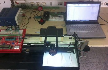
• Pen plotter mechanism.
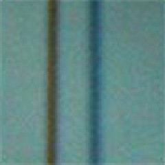
Fig 6: Original test image
Fig 4: The proposed mechatronic color registration system
Image investigation is carried out for the proposed color segmentation algorithm on the original image (test image). It is the image data was captured for the selected test printed sheet. The algorism is presented in
two phases (see Figure 5).
Phase 1: Original image input and pre-segmentation stage.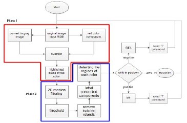
Phase 2: Image enhancements and color segmentation stage including investigation for step by step study.
Fig 5: The image analysis work flow diagram
The first phase of the algorithm is inputting the original file (image data) in RGB color space (Red, Green and Blue). The original image data is understood by the algorithm as a 3-dimensional matrix.
3.1.1 Original Test Image
The original test image (see Figure 6) gives a clear idea of how much noise and lake of details and quality which needs many enhancements to be clearly recognizable through the entire image analysis algorithm.
The noise in the image is due to the following reasons [4]:
• The compression of the image data format as it is in JPEG image data format. The name "JPEG" stands for Joint Photographic Experts Group, the name of the committee that created the JPEG standard and also other still picture coding standards.
• Lighting conditions: the lake of lighting in some video frames may result a noise in captured image.
• Lens focus: if the target object is out of focus it may become blurry which require more working on color segmentation in future pro- cessing.
All the mentioned reasons of image poor quality can be avoided when setting up the system. In other words, a more advanced camera can be deployed. Increasing the lighting quality can also help. However image enhancements will still be needed after all. No much effort will be done at this point as the algorithm will fix the problem in the coming stages.
The histogram plot of the original image (RGB) created in ABOBE PHOTOSHOP software (see Figure 7). The graph indicates that numbers of pixels of green and blue colors are almost the same while the pixels of red color are less to almost the half which will be easier for color seg- mentation to detect the red color with much less enhancements and rough operations. That’s why the original looks blue-green filtered (cyan overlay).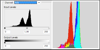
Fig 7: Photoshop histogram plot of the original image
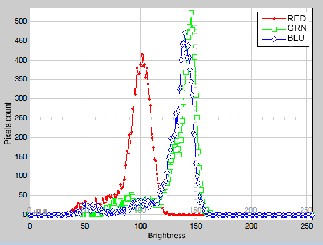
However, the plot under Photoshop environment can’t be merged through future investigation and calculation in the presented algorithm. So it is mentioned as a reference work and kept for comparison with MATLAB results. By calculating and plotting the histogram graph of the sample image was carried out in SIMULINK model. The graph of the tri-colors (Red-Green and Blue) shows that the red color is less count and brightness rather than the green and blue colors, which are almost the same brightness and pixel count. (see Figure 8).
IJSER © 2014 http://www.ijser.org
International Journal of Scientific & Engineering Research, Volume 5, Issue 9, September-2014 7
ISSN 2229-5518
Fig 11: Intensity plot of the gray image
Fig 8: Simulink histogram plot of original image
3.1.2 Gray Scale Image

Converting the tri-color image RGB to the grayscale intensity image is eliminating the hue and saturation information while retaining the lumi- nance (see Figure 9).
Fig 9: Gray image sample
For each pixel, the following equation (1) is used to calculate the intensi- ty [1][5]:
I = 0.2989 * R + 0.5870 * G + 0.1140 * B (1)
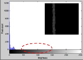
3.1.2.1 Gray Image Histogram Plot
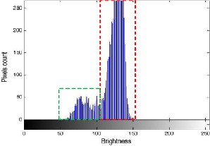
The histogram plot of the intensity map (gray scale image) shows that the gray image is consisting of two main regions of different data. The first region is the two color lines marked with green rectangle that obvi- ously have intensity values between 50 and 100 on the gray scale. While the rest is the background data marked with red rectangle which have intensity values between 100 and 150 (see Figure 10).
Fig 10: The two main regions of the histogram plot
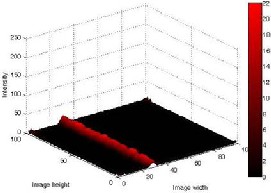
3.1.2.2 Gray Image Intensity Plot
By drawing the intensity plot, it is found that the red and blue line posi- tions are almost equal in intensity (see Figure 11). The intensities of both colors are almost below the 90 out of 255 (i.e. less than 35 %).
3.1.3 Image Data Array Subtractions
The subtraction of two images is performed straightforwardly in a single pass. The output pixel values are given by the following equation (2).
C(i,j)=A (i,j)–B(i,j) (2)
Where:
A... Gray image of the tricolor sample.
B... Single color vector image needs to be extracted.
i… Row number of the array and increments downwards. j… Column number of the array and increment rightwards.
If the pixel values in the input images are actually vectors rather than scalar values (i.e. for color images) then the individual components (i.e. red, blue and green components) are simply subtracted separately to produce the output value.
3.1.3.1 Image Subtraction Histogram Plot
In the histogram plot of the resulting image after performing the ubtracttion operation (see Figure 12), the range of intensities shown in the red highlighted area denoted as the noise region. This region should be compared with the histogram plot after applying the median filter in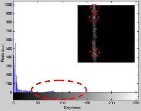
the next section.
Fig 12: Histogram plot after subtracting the red component out of the gray image
(the highlighted region is the noise values needs to be eliminated)
3.1.3.2 Image Subtraction Intensity Plot
The subtraction operation is performed and the resulting intensity is plotted (see Figure 13). The marked peaks also can be found in the his- togram plot (see Figure 12) will not result in a more correct thresholding in the next procedure.
IJSER © 2014 http://www.ijser.org
International Journal of Scientific & Engineering Research, Volume 5, Issue 9, September-2014 8
ISSN 2229-5518
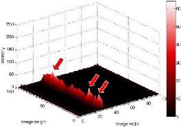
Fig 13: Intensity plot of subtraction operation
The process of information extraction from an image is known as image analysis. The first step in image analysis is the image segmentation [4]. It is the operation at the threshold between low-level image processing and image analysis. As a result, an image is segmented (classified) into a set of homogeneous and meaningful regions or objects, where each im- age pixel should belongs to an object. The core of the proposed segmen- tation scheme is to utilize each image pixel based on color values (color- based). Once the color regions are detected, rectangular boundaries rep- resent initial regions for the image. Next, the image is segmented into regions that correspond to each color.
3.2.1 Median Filter
Unlike the mean filter, the median filter is non-linear. This means that for two images A(x) and B(x):
median[A(x)+B(x)] ≠ median[A(x)]+median[B(x)] (3)
So, the smoothing is better performed to the directly analyzed image for more proper calculation [5].
3.2.1.1 Median Filter Histogram Plot
The histogram is plotted for the resulting image array after applying the median filter. The marked red area shows that non-uniform peaks are eliminated (see Figure 14).
Fig 14: Histogram plot after application of 2D median filter
3.2.1.2 Median Filter Intensity Plot
Smooth and uniform color locating in the sample image array is present- ed using the 2D median filter (see Figure 15).
Fig 15: Intensity plot after applying the 2D median filter
3.2.2 Region Labeling
A simple but powerful tool for identifying and labeling the various ob- jects in a binary image is a process called region labeling, blob coloring, or connected component identification. It is useful since once they are individually labeled, the objects can be separately manipulated, dis- played, or modified.
Region labeling seeks to identify connected groups of pixels in a binary image f that all have the same binary value. The simplest such algorithm accomplishes this by scanning the entire image (left to right, top to bot- tom), searching for occurrences of pixels of the same binary value and connected along the horizontal or vertical directions. The algorithm can be made slightly more complex by also searching for diagonal connec- tions, but this is usually unnecessary [3].
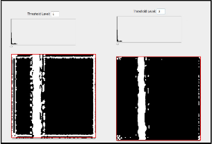
3.2.3 Adaptive Threshold Approach
A proposed method that is relatively simple, does not require much spe- cific knowledge of the image, and is robust against image noise, is the following iterative method:
1. An initial threshold (T) is chosen; this can be done randomly or according to any other method desired.
2. The image is segmented into object and background pixels as described above, creating two sets:
G1 = I(i,j)![]() T (object pixels)
T (object pixels)
G2 = I(i,j)![]() T (background pixels)
T (background pixels)
I(i,j) is the value of the pixel located in the ith column, jth row
3. The average of each set is computed.
m1 = average value of G1
m2 = average value of G2
4. A new threshold is created that is the average of m1 and m2
T’ = (m1 + m2)/2
Using the new threshold computed in step four, we keep repeating until the new threshold matches the one before it (i.e. until convergence has been reached). After reviewing the threshold figures (see Figure 16,17 and 18) we can tell that for certain, the number of the resulting bounding box (marked in red) around the object pixels (white pixels) is a way to select the proper threshold value which will be easy to check over it in a loop to insure a suitable value which will be more than 500 pixels and less than 1000 pixels (100 pixels * 10 pixels). For the example in hand, when the threshold value was set to be 10 bringing up 800 pixels (100 pixels height * 8 pixels) (see Figure 18), It will be a reasonable amount of correct object pixels to move on for the future algorithm procedures.
IJSER © 2014 http://www.ijser.org
International Journal of Scientific & Engineering Research, Volume 5, Issue 9, September-2014 9
ISSN 2229-5518
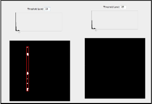
Fig 16: Threshold values taken under estimation
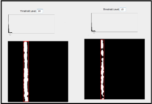
Fig 17: Threshold values taken over estimation
Fig 18: Threshold values taken into the acceptable range
As a self learning approach, the final threshold value detected from the last inspected image will then be the next start up value for the coming image so it is faster to detect the optimum threshold value for each im- age.
(Table 1) shows pixel count of the object bounding box for each thresh- old value. Also it shows the corresponding width and height of the bounding box.
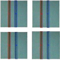
To be sure that the resulting segmentation is going well. It is necessary for the proposed algorithm to show the results of the color segmentation process. By applying the resulting boundaries to the original image cap- tured (color image) (see Figure 6). In other word, by putting the original image as a background to the bounding boxes resulting from both colors segmentation process (see Figure 19).
Fig 19: Examples of color segmented sample frames
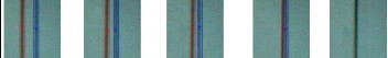
Finally, the difference in position between the two colors Centroids is calculated. According to the difference value, a command is sent via serial port to order the DC motor to correct the deviation detected. The deviation between the two printing colors continues to be reduced as the feeding goes forward. This operation will be stopped automatically when both color lines are positioned directly over each (see Figure 20).
Fig 20: Colors position deviation reduction through the correction process
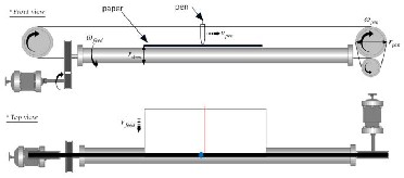
In order to study the mechatronic system, a mechanical model was re- constructed. The mechanical system dimensions and parameters were measured from the given system (see Figure 21). That was carried out to calculate the operation velocity of the feeding motor and the pen motor according to the given motor speed and the dimension of motion carriers (wires, belts, gears…etc.).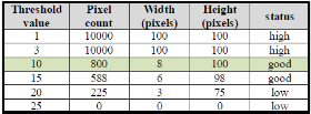
Fig 21: Mechanical system construction model
IJSER © 2014 http://www.ijser.org
International Journal of Scientific & Engineering Research, Volume 5, Issue 9, September-2014 10
ISSN 2229-5518
From the measured mechanical dimensions and the given motor speeds. Pen lateral motion speed and the feeding speed can be calculated using the equations:
vpen = ωPen . rPen
vfeed = ωdrum . rdrum
The proposed algorithm was built to automate the color registration pro- cess. It is important to monitor the wasted material due to the unregis- tered printed sheets. A simulation for the overall system characteristics was carried out to estimate the unregistered printed distance.
For the proposed system, there are three main factors affecting the wast- ed paper amount. These factors are:
• Feeding motor speed.
• Second color correction motor speed in lateral direction.
• Geometrical deviation amount between both two colors.
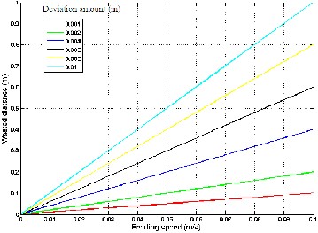
A simulation was carried out under MATLAB environment using Sim- ulink to estimate the resulted wasted amount of paper distance. The amount of unregistered printed sheets in terms of the distance travelled until the correction process was completed (see Figure 22). The wasted distance was drawn against the feeding speed for various deviation amounts. Geometrical deviation amount taken in the simulation was 1 mm as the smallest value and 10 cm as the largest one. Assuming a con- stant correction speed equal to 10 mm/s.
Fig 22: Wasted distance against feeding speed for various deviation amounts
In this paper, authors presented an approach to detect and correct the geometrical deviation of two over printed colors using computer vision technology. A pen plotter was implemented with mechatronic system based on vision system. Testing the algorithm and study its behavior is presented. Authors also Implemented MATLAB image processing toolbox to develop a technique to identify both colors with high accuracy and minimize computational time. Adaptive threshold value selector was tested in color segmentation and it showed more dynamic and flexibility to the color extraction process. Several typical tests are carried out that revealed good results and showed the applicability of the presented algo- rithm.
The potential of the proposed system can be further enhanced through the following suggested points:
• Improving the image sensor resolution in order to reduce the computa- tional time and increase the system accuracy.
• Replace the laptop computer as well as the microcontroller with an onboard computer as an embedded system. It can offer a stand-alone feature of the automation process.
• Use a suitable controller as PID controller or predictive controller to enhance the actuator behavior
• A system modification can be made in order to alert the operator when defect is detected.
[1] H. Kipphan, 2001 “Handbook of Print Media Technologies and Production
Methods”.
[2] H. Kipphan, 1993 “Quality and Productivity Enhancement in Modern Offset
Printing”.
[3] Elias N. Malamas, Euripides G.M. Petrakis, M. Zervakis, L Petit and Jean- Didier Legat, “A Survey on industrial vision systems, applications and tools”.
[4] Brosnan, 2004 “Improving Quality Inspection of Food Products by Computer
Vision”, Journal of food engineering.
[5] A. Bovik, 2000 “Handbook of Image and Video Processing”.
[6] J. Besl, L. Watson, 1988 ”Robust Window Operators”, International
Conferance on Computer Vision (ICCV), 1988.
[7] A. Marion, 1991”An Introduction to Image Processing”.
IJSER © 2014 http://www.ijser.org