International Journal of Scientific & Engineering Research, Volume 4, Issue 12, December-2013 208
ISSN 2229-5518
Two Algorithms Based on Shooting Method for
Solution of Falkner-Skan Equation
Dr. Gunindra Chandra Sarma, Mr. Dhrubajyoti Sarma
Abstract— Two algorithms based on shooting method have been developed, one for the solution of the Falkner-Skan [1] equation representing boundary layer flow past a wedge of angle β × π and the other for estimating the parameter β occurring in the governing equation. The numerical results agree upto 3 decimal places with the results obtained by previous authors using other numerical methods for the particular values β=0,1/2,1 and numerical results for β=-0.1988 are presented in table.
Index Terms— Algorithm. Shooting Method, Falkner-Skan Equation, boundary layer, similarlty variable, initial value problem, boundary value problem, viscous fluid.
1 INTRODUCTION
—————————— ——————————
The following equation known as Falkner-Skan [1] equation
f’’’ +f f’’ + β (1- f’2 ) =0 (1) Under the boundary condition
f(0) = 0 , f’(0) = 0 , f’ (∞)=1 (2)
y(p) (xf ) = yf (p) , p is any one 0,1,2 (4)
where the upper index p denotes the order of differentiation with respect to x and the lower index 0 for initial point and f for final point. That is we are considering the problem with two boundary conditions at the initial point and one boundary condition at the final point. We use here the initial value
IJSEmethod for solviRng ordinary differential equation. But in order
represents the flow of viscous fluid past a wedge of angleβ.
This equation was derived by Falkner-Skan [1] using dimen-
sionless similarity variables in the boundary layer equations
describing flow past a wedge. The equation is third order qua-
si linear and two conditions are specified at argument = 0 while one condition at argument = 1.
In this paper we present two algorithms one for the solu- tion of Falkner-Skan [1] equation and the other for estimating the parameter  and finally a numerical solution based on shooting method is presented.
2 SHOOTING METHOD
The Shooting method [2] is an advanced sophisticated com- puter oriented numerical method for solving boundary value problems. Let us consider a general two point third order boundary value problem. In all third order boundary value problem two boundary conditions are prescribed in one end point and another boundary condition at the other point. Without loss of generality let us assume that two boundary conditions are prescribed at the initial point x = x0 and one boundary condition at the final point x=xf (the problem pre- scribed with two boundary conditions at the final point and one condition at the initial point can be treated similarly by backward interpolation.
Let the general third order two-point boundary value problem be
to do so we must know all the initial conditions needed. Since
one of y0 (p) (p=0,1,2) is missing at x=x0, let it be an unknown pa- rameter λ(say) which must be so determined that the resulting
solution yields the prescribed final value yf (p) (p = 0, 1, 2) at x=xf to some desired accuracy.
Let λ0 and λ1 be guess values of the missing initial condition y0 (p) (x0 ) ( p takes the value 0, 1,2 which is not in the given ini- tial condition). Let y(P) (xf ,λ0 ) and y(P) (xf ,λ1 ) be the values of y(p)(xf ) ( p is given to be any one of 0,1,2) for λ=λ0 and λ=λ1 respectively obtained on integration of the initial value prob- lem for (3) in which λk (k=0,1)is taken as the missing initial condition. Then geometrically a better approximation λ2 of λ can be obtained as follows.
y’’’ = f(x, y, y’, y’’) (3)
With boundary conditions y(p) (x0 ) = y 0 (p), p is any two of 0,1,2
And
λ0 λ2 λ1
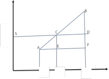
Fig 1: Linear interpolation of Guess Values
IJSER © 2013 http://www.ijser.org
International Journal of Scientific & Engineering Research, Volume 4, Issue 12, December-2013 209
ISSN 2229-5518
Let the points A and B in the Fig.1 represents the value of y(p)(xf ) when λ = λ0 and λ = λ1 respectively, when y(p)(xf ) is plotted against λ. Let SD be the line y(p)(x f ) = y(p) f
then a better approximation of λ2 of λ can be obtained by line- ar interpolation given by
λ2 = λ0 + (λ1 – λ0 ) { y(p) f - y(p) ( xf , λ0 )} / { y(p) ( xf , λ1 ) - y(p) (
xf , λ0 )} (5)
(from the similar triangles CAE and BAF). Now (3) can be in- tegrated with the two given initial conditions and λ2 as the missing initial condition to obtain y(p) ( xf , λ2 ). Again using linear interpolation based on λ2 and λ1 we can obtain the next approximation λ3 . The process is repeated until y(p) ( xf , λk ) = y(p) f is satisfied to some desired accuracy for some k.
Convergence of the iteration process described above is not guaranteed. But once the chosen value is nearer to the true value the convergence is very rapid.
The shooting method has tremendous applications in solving boundary value problems. It is also applied to three- point double parametric boundary value problems by various au- thors. We have developed a general algorithm to solve (3) to
(4) which which we have described in the next section.
- y(p) ( xf , λk )} and go to step 2.
Step 6: Solve the problem using two given initial condition and λk is the missing initial condition and stop. (though the convergence is not guaranteed at present in the iteration pro- cess described above, it appears in practice that it is very rapid if the two guessed values are in opposite sides of the true val- ue. Otherwise also, when the chosen value is nearer to the true value the process converges rapidly).
The algorithm may be applied to almost all two-point boundary value problems whose order is higher than three provided that only one condition from the minimum number of required initial conditions at one end point is missing.
4 APPLICATION OF ALGORITHM TO (3) TO (4)
Since it is not easy to form an analytical method to look for the guess values, in our present problem we consider a particular value of β and try to get two guess values say λ0 and λ1 for the missing initial condition f’’(0) corresponding to that value of β. In this selection a trial and error method is used. It is experi- enced that once the inaration method is convergent with above λ0 and λ1 for that value to β, the selection of the guessed
values corresponding to any other value of β becomes much
IJSEeasier. R
3 NUMERICAL SOLUTIONS
Due to nonlinearity of the problem (3) to (4) a closed form so- lution is not possible to obtain. Hence numerical solutions of the problem are essential. Based on the shooting method of a general algorithm has been developed to solve (3) to (4).
3.1 Algorithm
Step1 : Let λk be the approximation for the unknown initial condition y(p) ( x0 ) = y0 (p) , p is any one of 0,1,2 and takes the value which is not in the other prescribed conditions. (λ0 , λ1 can be chosen from physical consideration of the problem or by a trial and error method).
Step2: Solve the initial value problem
Y’’’ = f (x, y, y’, y’’)
y(p) ( x0 )= y0 (p) , p is any two of 0,1,2 which are prescribed and y(p) (x0 )= λk , k= 0,1 .... and p is any one of 0,1,2 which are not in the prescribed conditions from x=x0 to x=xf using any
method for solving initial value problems.
Step3: Call y(p) (x f , λk ) , (k=0,1,.....) the value of yp (xf ) ( p is any one of 0,1,2 which is given ) obtain on integration the ini- tial value problem in Step – 2.
Step 4: If │y(p) f – y(p) (xf , λk )│< ε for a tolerable ε, then go
to step 6 otherwise continue.
Step 5: Obtain the next approximation for the unknown ini- tial condition from
λk+2 = λk + (λk+1 – λk ) { y(p) f - y(p) ( x f , λk )} / { y(p) ( xf , λk+1 )
Since in (3) to (4) one of the boundary is η=∞, the problem be- comes a singular one. The boundary η=∞ is tackled in the fol- lowing manner. First for the fixed β, a large value η= η∞ (say) is chosen and corresponding initial condition f’’(0) is deter- mined. Let this estimated value of f’’(0) be λi . We go on in- creasing the value of η∞ after estimating f’’(0) at each value until a fixed value of f’’(0) is attained. Then say η∞ for which f’’(0) takes that fixed value is considered as the truncated boundary for η=∞. If the guessed value to η∞ is large enough ( say 5 here) the process for determining the boundary η=∞ is not repeated more than two times.
5 ESTIMATION OF THE PARAMETER Β BY SHOOTING
METHOD
It has been possible to estimate the parameter by Shooting Method. Knowing all the initial conditions the parameter β can be estimated in such as way that the resulting estimation satisfy f’(∞)=1 to some desired accuracy in a similar manner to that of estimation of f’’(0).
Since f’(∞) is a function of β a similar geometry can be con- structed by plotting f’(∞) against β. If β0 and β1 are approxi- mate values of β for f(0) = 0 , f’(0) =0 and for fixed f’’(0) = ∞ (say) then the corresponding iteration formula for the next approximation β2 of β are given by
β2 = β0 + (β1 – β0 ) { 1 - f’( ∞ , β0 )} / { f’ ( ∞ , β1 ) – f’ ( ∞ , β0 )} (6)
where we put f’(∞) = 1 and f’ (∞,βk ), (k= 0,1) are the values
IJSER © 2013 http://www.ijser.org
International Journal of Scientific & Engineering Research, Volume 4, Issue 12, December-2013 210
ISSN 2229-5518
of f’(∞) obtained on integration the initial value problem with f’’(0) = ∞ (known) and β = βk . Then using β = β2 , the equation is again integrated to obtain f’ (∞,β2 ) and linear iteration based on β1 and β2 a better approximation β3 can be obtained. The process is repeated until the resulting approximation of β satisfied f’(∞) = 1 to some desired places.
Here also the convergence of the iteration process is not guaranteed but once the chosen value is nearer to the true val- ue the process converges very rapidly. Also if the two guessed values are in opposite sides of the true value the convergence is very rapid.
Accordingly we have presented below an algorithm for es-
timation of β.
5.1 Algorithm
Step 1 : let β0 and β1 be two approximate values of for some
known f’’(0) = ∞ (say).
Step 2: integrate the initial value problem
f’’’ + f f’’ + βk (1- f’2 ) = 0
with f(0) = 0 , f’(0) =0 , f’’ (0) = ∞, k= 0, 1, ....
from η = 0 to η = ∞ ( the boundary η = ∞ is now easy to de-
Hence the critical value of β is such that, for that particular value of β, f’’(0) = 0 holds. So one can estimate β for which f’’(0) = 0.
It is not easy to get an analytical expression for A (β) , which satisfies A (β) = 0, so that the critical value of β can be determined. Also we are in a position to estimate the parame- ter β for known f’’(0), so we take the second approach, to de- termine the least value of β. Using the second algorithm for f’’(0) =0, we obtain β = - 0.19884 which is the critical value of the parameter β.
7 RESULTS AND DISCUSSIONS
The two guessed values needed for the algorithms to estimate f’’(0) and β are chosen by trial and error methods. Once the correct values are obtained for some cases e.g. for some pre- scribed β in estimation of f’’(0) and for some prescribed f’’(0) in estimation of β then it becomes easier to choose the guess values for any other values of β or f’’(0) as the case may be.
The values if f, f’ and f’’ for β = 0, ½, 1 obtained by shooting method agree up to three places of decimal with those of Blasius [3], Frossling [4] and Hiemenz [5]. For β = -0.1988, values of f, f’ and f’’ are presented in table.
termine for known f’’ (0).
IJSER
Step 3: Call f’ (∞ , βk ) the value of f’(∞) obtained from step
2 on integration with β=βk ,
Step 4 : if │1- f’ (∞,βk )│< ε for some prescribed ε, then go to
step 6 otherwise continue.
Step 5: Obtain next approximation from
βk+2 = βk + (βk+1 – βk ) { 1 - f’ ( ∞ , βk )} / { f’ ( ∞ , βk+1 ) – f’ (
∞ , βk )} and go to step 2.
Step 6: Solve (2.1) as initial value problem with f(0) = 0, f’(0)
= 0, f’’(0) = ∞ , β=βk and stop.
We have tested the algorithm for some known f’’(0) and known β. Then it becomes easier to guess the two values of β for any other values of f’’(0). The boundary η=∞ is now very easy to tackle.
6 LOWER BOUND OF 
It is proved analytically that the upper bound of does not exist. For β< 0, f’’ (0) satisfies the inequality (2.3). For problem (2.1) to (2.2), the number a defined in section 2.3 depends only on β, and (2.3) takes the form 0 ≤ f’’(0) ≤ h(0) since a = 0 here. Therefore the critical value of β is related to the condition f’’(0)
= 0. There are two ways to determine the least value of β for which solution of (2.1) and (2.2) exists. Firstly the number A should be chosen in such as way that A(β) = 0.
Then solving this equation for β one can obtain the least value of β. Secondly, if A (β) = 0 holds, then by definition of h, h(A) = h(a) = h(0) = 0 and hence f’’(0) =0 for the least value of β.
REFERENCES
[1] Falkner, V.M., Skan, S. W., “Some Approximate Solutions of the Boundary
Layer Equation”, Philosophical Magazine, vol 12, 865-896.
[2] Conte, S. D., “Elementary Numerical Analysis – An Algorithmic
Approach”, McGrawHill Book Co, New York, 1965.
[3] Blasius, H., “Grenzschichten Flϋssigkeiten mit kleiner Reibung. Z.
Math u Phys”, 1908, vol 56, 1-37
[4] Frössling, N., Verdunstung, “Wӓ rmeubertragung und Geschwindigkeitsverteilung bei zweidimensionaler und rota- tionssymmetrischer laminarer Grenzschichtströmung Lunds”, Uni- versity Arsskr. N.F.,1940, Adv 2, 35, No 4.
[5] Hiemenz, F., “Die Grenzschicht an einem in den gleichförmigen Flussigkeitsstrom eingetauchten geraden Kreiszylinder. ( Thesis Göt- tingen 1911)”, Dingl. Polytechnique Jounral 326, 321 (1911).
[6] Bairstow, L., “Skin Friction”, Journal of Royal Aeronautical Society,
1925, vol 19, 3.
[7] Collatz, L.,“Numerical Treatment of differential equations”, Springer
Verlag inc, New York, 1966.
[8] Goldstein, S., “On the Two Dimensional Steady Flow of a Viscous
Fluid Behind a Solid Body”, Proceedings of Royal Society London,
1933,A 142, 545-562
[9] Goldstein, S., “A Note on Boundary Layer Equation”, Proceedings of
Cambridge Philosophical Society, 1939, vol 35, 388-340.
[10] Goldstein, S., “Modern Development in Fluid Dynamics”, Clarendon
Press, Oxford, 1938,Vol I, 105.
[11] Hartree, D. R., “On an Equation Occurring in Falkner and Skan’s Approximate Treatment of the Equations of the Boundary Layer”, Proceedings of Cambridge Philosophical Society, 1937,vol 33, Part II,
223-239.
[12] Homann, F., “Der Einfluβ Groβer Zӓ higkeit bei der Strömung um
den Zylinder und um die Kugel”, 1936,ZAMM 16, 153-164.
IJSER © 2013 http://www.ijser.org
International Journal of Scientific & Engineering Research, Volume 4, Issue 12, December-2013 211
ISSN 2229-5518
[13] Howarth, L., “On the Calculation of the Steady Flow in the Boundary Layer
near the Surface of a Cylinder in a Stream”, 1935,ARC R M 1632.
[14] Howarth, L., “On the Solution of the Laminar Boundary Layer Equa-
tions”, Proceedings of Royal Society London, 1938,A 164, 547-579.
[15] Mangler, W., “Die ӓ hnlichen Lösungen der Prandtlschen
Grenzschichtgleichungen”, 1943,ZAMM 23, 241-251.
[16] Meksyn, D., “Integration of Boundary Layer Equation”, Proceedings of
Royal Society London, 1956,A 237, 543-559.
[17] Meksyn, D., “New Methods in Laminar Boundary Layer theory”,
1961,Pergaman Press London.
[18] Roberts, S.M. and Shipman, J.S. , “Two Point Boundary Value Problems – Shooting Methods”, American Elsevier Company, New York (1972).
[19] Scarborough, J.B., “Numerical Mathematical Analysis”, Oxford and IBM
publishing Company, New Delhi,1966.
[20] Stewartson, K., “Further Solution of the Falkner-Skan Equation”, Proceed-
ings of Cambridge Philosophical Society, 1954,vol 50, 454-465.
[21] Töpfer, C., Bemerkungen zu dem Aufsatz von H Blasius, “Grenzschichten
Flϋssigkeiten mit kleiner Reibung”, 1912,Z. Math. U. Phys., 60, 397-398.
IJSER
IJSER © 2013 http://www.ijser.org
International Journal of Scientific & Engineering Research, Volume 4, Issue 12, December-2013 212
ISSN 2229-5518
Appendix A
β=-0.1988
IJSER
IJSER © 2013 http://www.ijser.org