The research paper published by IJSER journal is about Time Synchronization in Wireless Sensor Networks 1
ISSN 2229-5518
Time Synchronization in Wireless Sensor Net- works
Shashank Bholane, Devendrasingh Thakore
Abstract— W ireless Sensor Networks (WSNs) consists of numerous small sensors. These sensors are wirelessly connected to each other for perfor m- ing same task collectively such as monitoring weather conditions or specifically parameters like temperature, pressure, sound and vibrations etc. For all applications partial or full time synchronization is required and the message exchanged by sensor nodes for data fusion must be time stamped by each sensor’s local clock. This helps to achieve a common notion of time in wireless sensor networks. This paper contains a survey, relative study and analy- sis of existing time synchronization protocols for wireless sensor networks, based on various parameters. No single protocol is optimal and suff icient in all aspects for designing a clock synchronization system. So the comparative study and design considerations will help a lot to the designer for designing a scheme which may or may not be application specific.
Index Terms— Time synchronization, W ireless sensor networks, Protocol
—————————— ——————————
n recent years, wireless sensor network, has received much attention of researchers as the technological advancement has made these low power devices very cost effective. Wire- less sensor networks consist of numerous tiny low-power de- vices capable of performing sensing and communication tasks
collectively.
Wireless sensor networks were first deployed for military applications. Gradually researchers found them to be very useful in applications like weather monitoring, habitat moni- toring, agriculture, industrial applications, and recently smart homes and kindergartens [1, 2]. Wireless sensor network is an ad hoc network and being distributed in nature, time syn- chronization becomes a critical part of its functioning. Every small sensor consists of an embedded processor, memory and radio. Precise and synchronized time is needed for several reasons. For example, an accurate and synchronized time is necessary to determine the right chronological order of events as in target tracking. A lack of synchronization may lead to incorrect time stamping and misinterpretation of the readings.
For a wired network, two methods of time synchronization are most common. Network Time Protocol (NTP) [3] and Global Positioning System (GPS) are both used for synchroni- zation. Neither protocol is useful for wireless sensor synchro- nization [4]. Both require resources not available in wireless networks. The Network Time Protocol requires an extremely accurate clock, usually a server with an atomic clock. The client computer wanting to synchronize with the server will send a UDP packet requesting the time information. The serv- er will then return the timing information and as a result the computers would be synchronized. Because of many wire- less devices are powered by batteries, a server with an atomic clock is impractical for a wireless network. GPS requires the
————————————————
![]() Devendrasingh M. Thakore is currently working as a professor in computer
Devendrasingh M. Thakore is currently working as a professor in computer
engineering department in bharati vidyapeeth deemed university, I ndia. E-
mail: deventhakur@yahoo.com
wireless device to communicate with satellites in order to syn- chronize. This requires a GPS receiver in each wireless device. Again because of power constraints, this is impractical for wireless networks. Also sensor networks consist of inexpen- sive wireless nodes. A GPS receiver on each wireless node would be expensive and therefore unfeasible. The time accu- racy of GPS depends on how many satellites the receiver can communicate with at a given time. This will not always be the same, so the time accuracy will vary. Furthermore Global Posi- tioning System devices depend on line of sight communication to the satellite, which may not always be available where wire- less networks are deployed.
The constraints of wireless sensor networks do not allow for traditional wired network time synchronization protocols. Wireless sensor networks are limited to size, power, and com- plexity. Neither the Network Time Protocol nor GPS were de- signed for such constraints.
For a wireless sensor network, there are three basic types of synchronization methods. The first is relative timing and is the simplest. It relies on the ordering of messages and events. The basic idea is to be able to determine if event 1 occurred before event 2. Comparing the local clocks to determine the order is all that is needed. Clock synchronization is not impor- tant.
The next method is relative timing in which the network clocks are independent of each other and the nodes keep track of drift and offset. Usually a node keeps information about its drift and offset in correspondence to neighboring nodes. The nodes have the ability to synchronize their local time with another nodes local time at any instant. Most synchronization protocols use this method.
The last method is global synchronization where there is a constant global timescale throughout the network. This is ob- viously the most complex and the toughest to implement. Very few synchronizing algorithms use this method particu- larly because this type of synchronization usually is not neces- sary.
IJSER © 2012
The research paper published by IJSER journal is about Time Synchronization in Wireless Sensor Networks 2
ISSN 2229-5518
Time synchronization schemes have four basic packet delay components: send time, access time, propagation time, and receive time [5]. As shown in Fig.1 the send time is that of the sender constructing the time message to transmit on the net- work. The access time is that of the MAC layer delay in access- ing the network. This could be waiting to transmit in a TDMA protocol. The time for the bits to by physically transmitted on the medium is considered the propagation time. Finally, the receive time is the receiving node processing the message and transferring it to the host.
Sender Propagation Receiver
for wireless sensor networks. There are other synchronization protocols, but these three represent a good illustration of the different types of protocols. These three cover sender to re- ceiver synchronization as well as receiver to receiver. Also, they cover single hop and multi hop synchronization schemes.
Many of the time synchronization protocols use a sender to receiver synchronization method where the sender will transmit the timestamp information and the receiver will syn- chronize to sender. RBS is different because it uses receiver to receiver synchronization. The idea is that a third party will broadcast a beacon to all the receivers. The beacon does not contain any timing information; instead the receivers will compare their clocks to one another to calculate their relative phase offsets.
The timing is based on when the node receives the refer- ence beacon. The simplest form of RBS is one broadcast bea- con and two receivers. The timing packet will be broadcasted
Send
Time
Access
Time
Propagation
Time
Receive
Time
to the two receivers. The receivers will record when the packet was received according to their local clocks. Then, the two receivers will exchange their timing information and be able to calculate the offset. This is enough information to retain a local
Fig. 1. Non-deterministic delay components
The major problem of time synchronization is not only that this packet delay exists, but also being able to predict the time spent on each can be difficult [6]. Eliminating any of these will greatly increase the performance of the synchronization tech- nique.
The authors have identified requirements for solving this problem [5, 6, 7]. These techniques aim to build a synchroniza- tion service that conforms to the requirements of WSNs:
Robustness: the service must continuously adapt to condi- tions inside the network, despite dynamics that lead to net- work partitions.
Energy efficiency: the energy spent synchronizing clocks should be as minimal as possible, because there is significant cost to continuous CPU use or radio listening.
Scalability: large populations of sensor nodes (hundreds or thousands) must be supported. Every application need differ- ent number of sensors deployed in sensor field.
Ad hoc deployment: time sync must work with no a priori configuration, and no infrastructure available
timescale.
RBS can be expanded from the simplest form of one broad- cast and two receivers to synchronization between n receivers; where n is greater than two. This may require more than one broadcast to be sent. Increasing the broadcasts will increase the precision of the synchronization. The reference beacon is broadcasted across all nodes. Once it is received, the receivers note their local time and then exchange timing information with their neighboring nodes. The nodes will then be able to calculate their offset [8].
This protocol uses a sequence of synchronization messages from a given sender in order to estimate both offset and skew of the local clocks relative to each other. The protocol exploits the concept of time-critical path, that is, the path of a message that contributes to non-deterministic errors in a protocol. Fig.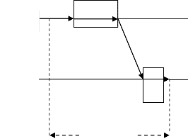
2 and Fig. 3 compare the time-critical path of traditional proto- cols, which are based on sender-to-receiver synchronization, with receiver-to-receiver synchronization in RBS.
NIC Sender
There are many time synchronization protocols, many of which do not differ much from each other. As with any proto- col, the basic idea is always there, but improving on the dis- advantages is a constant evolution. Three protocols will be discussed: Reference Broadcast Synchronization (RBS) [8], Timing-sync Protocol for Sensor Networks (TPSN) [9], and Flooding Time Synchronization Protocol (FTSP) [10]. These
Receiver
Critical Path
three protocols are the major timing protocols currently in use
Fig. 2. Traditional time synchronization
IJSER © 2012
The research paper published by IJSER journal is about Time Synchronization in Wireless Sensor Networks 3
ISSN 2229-5518
Sender
Receiver
NIC
An edge between two vertices in this graph exists if the corresponding nodes in the network are within the same neighborhood formed by RBS, i.e., if the two nodes can receive synchronization pulses from the same beacon sender. Then multi-hop synchronization can be performed along the edges of this graph. To this end, the concept of ―time routing in mul- ti-hop networks‖ is introduced. Finding the shortest path be- tween two nodes would yield a minimal error multi-hop syn- chronization path for this pair of nodes [8]. Moreover, the au- thors proposed assigning weights to edges to represent the quality of pairwise synchronizations (e.g., using the residual error of the linear fit). In the analysis of the multi-hop RBS algorithm, the authors argue that there is just a slow decay in precision by multi-hop synchronization; the average synchro- nization error is proportional to n for an n -hop network.
Critical Path
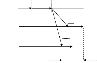
Fig. 3. RBS synchronization
The delays that occur at the sender side are eliminated by using the physical layer broadcast in sensor networks. The critical path now contains the propagation and the receiver uncertainty. If, however, the transmission range is relatively small, then we can eliminate the propagation time and the critical path only contains the uncertainty of the receiver [8].
In many cases, the nodes that need synchronized time may not be in the coverage area of some common node. Then, some other nodes should act as gateways for time translation be- tween neighborhoods to route the time information from one node to another.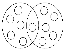
Fig. 4. depicts a case where multi-hop synchronization is required. For example, node 1 and node 7 are not in the same neighborhood, i.e., they do not share a common sender from which they can both receive a synchronization pulse. In this case, node 4 acts as a gateway node between the two neigh- borhoods. When senders A and B broadcast synchronization pulses to their neighborhood as usual, node 4 gets both of these pulses and can thus relate the local clocks of A and B, i.e., the two neighborhoods. When a beacon sender broadcasts a synchronization pulse, it essentially creates a set of nodes (a neighborhood) in which nodes can relate their local clocks among each other. Now consider a graph whose vertices cor- respond to sensor nodes in the network.
TPSN is a traditional sender-receiver based synchronization. It uses a tree to organize the network topology. The working of protocol is split into two phases, the level discovery phase and the synchronization phase. The level discovery phase creates the hierarchical topology of the network. In this phase each node is assigned a level. Only one node, the root, resides on level zero. In the synchronization phase every i level node will synchronize with i-1 level nodes. This will result in all nodes synchronized with the root node [9].
Level Discovery Phase: In the level discovery phase the root node should be assigned first. If one node was equipped with a GPS receiver, then that could be the root node and all nodes on the network would be synced to the world time. If not, then any node can be the root node and other nodes can periodical- ly take over the functionality of the root node to share the re- sponsibility. Once the root node is determined, it will initiate the level discovery. The root, level zero, node will send out the level_discovery packet to its neighboring nodes. In the lev- el_discovery packet, the identity and level of the sending node is included. The neighbors of the root node will then assign themselves as level one. They will in turn send out the lev- el_discovery packet to their neighboring nodes. This process will continue until all nodes have received the level_discovery packet and are assign a level.
Synchronization Phase: The root node starts this phase by broadcasting a time_sync packet. Upon its reception, the nodes on level 1 wait for a random time then send a synchroniza- tion_pulse packet to the root node. The randomized waiting prevents collisions caused by contention for media access. The
1 7
3 9
8 6
2 5
Fig. 4. Multi-hop RBS
root node replies accordingly with acknowledgement packets. Therefore, all nodes belonging to level 1 can correct their clocks according to the clock of the root node. In addition, the nodes on level 2 will overhear the two-way message exchange because they have at least a neighbor on level 1. Consequently, the nodes on level 2 will each send a synchronization_pulse packet to their level-1 neighbors for synchronization. This is applied recursively with nodes on level i synchronizing their clocks to nodes on level i-1. Eventually, every node in the network has its clock synchronized to the reference clock of
IJSER © 2012
The research paper published by IJSER journal is about Time Synchronization in Wireless Sensor Networks 4
ISSN 2229-5518
the root node, thus, the global clock synchronization is achieved.
Fig. 5. illustrates the two-way messaging between a pair of nodes. This messaging can synchronize a pair of nodes by fol- lowing this method. The times T1, T2, T3, and T4 are all meas- ured times. Node A will send the synchronization_pulse packet at time T1 to Node B. This packet will contain Node A's![]()
(T2-T1)-( T4-T3)
∆ =
2
(T2-T1)+( T4-T3)
d =
2
(1)
(2)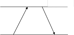
level and the time T1 when it was sent. Node B will receive the packet at time T2. Time T3 is when Node B sends the ac- knowledgment_packet to Node A. That packet will contain the level number of Node B as well as times T1, T2, and T3. By knowing the drift, Node A can correct its clock and successful- ly synchronize to Node B. This is the basic communication for TPSN.
Another form of sender to receiver synchronization is FTSP. This protocol is similar to TPSN, but it improves on the disad- vantages to TPSN. It is similar in the fact that it has a structure with a root node and that all nodes are synchronized to the root. The root node will transmit the time synchronization information with a single radio message to all participating
Node B
Node A
T2 T3 Local Time
receivers. The message contains the sender's time stamp of the
global time at transmission. The receiver notes its local time
when the message is received. Having the sender's transmis- sion time and the reception time, the receiver can estimate the
clock offset. The message is MAC layer time stamped, as in TPSN, on both the sending and receiving side. To keep high precision compensation for clock drift is needed. FTSP uses linear regression for this. FTSP was designed for large multi- hop networks. The root is elected dynamically and periodical-
T1
Fig. 5. Two-way messaging in TPSN
T4 Local Time
ly reelected and is responsible for keeping the global time of the network. The receiving nodes will synchronize themselves to the root node and will organize in an ad hoc fashion to
The synchronization process is again initiated by the root node. It broadcasts a time_sync packet to the level one nodes. These nodes will wait a random amount of time before initiat- ing the two-way messaging. The root node will send the ac- knowledgment and the level one nodes will adjust their clocks to be synchronized with the root nodes. The level two node will be able to hear the level one nodes communication since at least one level one node is a neighbor of a level two node. On hearing this communication the level two nodes will wait a random period of time before initiating the two-way messag- ing with the level one nodes. This process will continue until all nodes are synchronized to the root node. Again the syn- chronization process executes much the same as the level dis- covery phase. All communication begins with the root node broadcasting information to the level 1 nodes. This communi- cation propagates through the tree until all level i-1 nodes are synchronized with the level i nodes. At this point all nodes will be synchronized with the root node.
Here, T1, T4 represent the time measured by local clock of
‗A‘. Similarly T2, T3 represent the time measured by local
clock of ‗B‘. At time T1, ‗A‘ sends a synchronization_pulse packet to ‗B‘. The synchronization_pulse packet contains the level number of ‗A‘ and the value of T1. Node B receives this packet at T2, where T2 is equal to T1 + ∆ + d. Here ∆ and d represents the clock drift between the two nodes and propaga- tion delay respectively. At time T3, ‗B‘ sends back an acknowl- edgement packet to ‗A‘. The acknowledgement packet con- tains the level number of ‗B‘ and the values of T1, T2 and T3. Node A receives the packet at T4. Assuming that the clock drift and the propagation delay do not change in this small span of time, ‗A‘ can calculate the clock drift and propagation delay as:
communicate the timing information amongst all nodes. The network structure is mesh type topology instead of a tree to- pology as in TPSN. [10]![]()
Sender
Preamble Sync Data CRC

Propagation ![]() delay
delay
Preamble Sync Data CRC Receiver Byte alignment
Fig. 6. Data packets transmitted over the radio channel.Solid lines
represent the bytes of the buffer and the dashed lines are the bytes of packets.
There are several advantages to FTSP over TPSN. Al- though TPSN did provide a protocol for a multi-hop network, it did not handle topology changes well. TPSN would have to reinitiate the level discovery phase if the root node changed or the topology changes. This would induce more network traffic and create additional overhead. FTSP is robust in that is utiliz- es the flooding of synchronization messages to combat link and node failure. The flooding also provides the ability for dynamic topology changes. The protocol specifies the root node will be periodically reelected, so a dynamic topology is necessary. Like TPSN, FTSP also provides MAC layer time stamping which greatly increases the precision and reduces jitter. This will eliminate all but the propagation time error. It utilizes the multiple time stampings and linear regression to estimate clock drift and offset.
IJSER © 2012
The research paper published by IJSER journal is about Time Synchronization in Wireless Sensor Networks 5
ISSN 2229-5518
In this section we compare and evaluate the above discussed synchronization protocols. We need to define various evalua- tion criteria for qualitative and quantitative comparison of time synchronization protocols.
Here we evaluate the protocols based on overall quality crite- ria. The various protocols are compared in terms of the follow- ing qualitative criteria and are summarized in table 1 [6, 11].
1. Accuracy: A measure of the precision of synchronization. A protocol with high accuracy provides the guarantee of high precision. The absolute precision is achieved if the synchro- nized time in the network does not deviate much from an ex- ternal standard.
2. Energy Efficiency: In WSNs nodes are distributed in areas where it is impossible to wire these nodes to a power source. Draining the power of nodes will degrade the efficiency of the network. Therefore, Energy efficiency is an implicit require- ment in wireless sensor networks.
3. Scalability: Synchronization technique must work well with any number of nodes in the network. The synchronization protocols must be sufficiently scalable with varying network size. This is a limitation on many protocols as they are tested for a few hundred nodes.
4. Overall Complexity: In wireless sensor networks there is always limited resources and hardware capabilities and also have severe energy constraints. The complexity of protocol can make a protocol impracticable for many applications.
5. Fault Tolerance: Fault tolerance plays an important role be- cause in wireless medium there is more chance of errors. If the delivery of a message is poor in WSNs then it could lead to devastating effects on synchronization protocols. Some fault- tolerant protocols solved message loss problem to some level, but some protocols do not addressed this issue [9].
TABLE 1
QUALITATIVE METRICS AND PERFORMANCE OF TIME SYNCHRONIZA- TION PROTOCOLS
ristics and requirements of each application. For instance, a low cost, low precision protocol could be appropriate for many environmental monitoring applications. However, many safety critical applications, such as aircraft navigation or intrusion detection in military systems, will demand high pre- cision protocols in order for nodes to correctly identify events occurring in the network.
1. Precision: Synchronization precision can be defined in two ways: Absolute precision: The maximum error (i.e. skew and offset) of a node‘s logical clock with respect to an external standard such as UTC. Relative precision: The maximum dev- iation (i.e., skew and offset) among logical clock readings of the nodes belonging to a wireless network. Precision of syn- chronization technique highly depends on the application.
2. Convergence Time: Convergence time is the total time re- quired to synchronize the network.
3. Piggybacking: Piggybacking is a term used to describe the process of combining synchronization message with data mes- sage sent amongst nodes. Instead of sending independent ac- knowledgement messages, these messages are piggybacked on the data messages that have to be sent to the node, in order to reduce message traffic in the network.
4. Computational Complexity: As wireless sensor networks often have limited hardware capabilities and severe energy constraints, the complexity of a synchronization protocol can make a protocol impractical for many applications.
5. Graphic Users Interface Services: Graphic User Interface (GUI) services provide the ease to the end user. Only Ping‘s protocol [12] provides such services to the application and higher level kernel modules.
6. Network Size: Local synchronization technique must be extended to the entire network in WSNs. The network wide time synchronization protocol of Ganeriwal et al. [8] is impor- tant in this regard. This protocol was found to handle neigh- borhoods with up to 300 nodes.
Table 2 compares the various protocols in terms of the above discussed quantitative criteria [6, 11]. These qualitative and quantitative criteria can be used as metrics or perfor- mance measures to evaluate or analyse the trade off between various requirements on time synchronization protocols for wireless sensor networks.
TABLE 2
QUANTITATIVE METRICS AND PERFORMANCE OF TIME SYNCHRONI- ZATION PROTOCOL
The protocols mentioned in previous section differ in their computational requirements, energy consumption, precision of synchronization results, and communication requirements. In various applications of wireless sensor networks no single protocol is applicable for all applications. In WSNs one proto- col is suitable for one application but not fit for other applica- tion. The choice of a protocol will be driven by the characte-
IJSER © 2012
The research paper published by IJSER journal is about Time Synchronization in Wireless Sensor Networks 6
ISSN 2229-5518
We have discussed, analyzed and compared RBS, TPSN and FTSP protocol for time synchronization in WSN. This will help researchers and designers a lot in selection of time synchroni- zation protocol to build a system or an application where par- tial or full time synchronization is necessary. These protocols can be simulated in suitable network simulator and selection guideline can be refined.
[1] Mani B. Srivastava, Richard R. Muntz, and Miodrag Potkonjak.,‖Smart kin- dergarten: sensorbased wireless networks for smart developmental problem- solving environments‖. In Mobile Computing and Networking, pp. 132-138,
2001.
[2] I.-K Rhee, J Lee, J. Kim, E. Serpedin, Wu, Y.-C. ―Clock Synchronization in
Wireless Sensor Networks: An Overview‖. Sensors: pp 56-85, 2009
[3] D. L. Mills, ―Internet time synchronization: the network time protocol.‖ IEEE Trans. Commun. , 10: pp 1482-1493, 1991.
[4] I.. F. Akyildiz, W. Su , Y. Sankarasubramaniam and E. Cayirci., ―WirelessSen-
sor Networks: A Survey‖. Computer Networks, 38(4), pp.393422, 2002.
[5] F. Sivrikaya and B. Yener, ―Time Synchronization in Sensor Networks: A Survey,‖ Network, IEEE 18(4), pp.45–50, 2004.
[6] B. Sundararaman et al., ―Clock synchronization for wireless sensor net-
works: a survey,‖ Ad-Hoc Networks, vol. 3, no. 3, pp. 281–323, Mar.2005. [7] J. Elson and D. Estrin, ―Time Synchronization for Wireless Sensor N et-
works", International Parallel and Distributed Processing Symposium, San
Francisco, USA, 2001.
[8] J. Elson, L. Girod , and D. Estrin , ―Fine-grained network time synchroniza- tion using reference broadcasts‖ In Fifth Symposium on Operating Systems Design and Implementation OSDI, 2002.
[9] Saurabh Ganeriwal, Kumar Ram, and Mani B. Srivastava ―Timing-sync protocol for sensor networks‖. In First ACM Conference on Embedded Networked SensorSystems, SenSys, 2003.
[10] M. Maroti, B. Kusy, G. Simon, and A. Ledeczi, ―The floodi ng time syn- chronization protocol,‖ in Proc. Second International Conference on Em- bedded Networked Sensor Systems 2004, ACM Press, pp. 39–49, Nov.
2004.
[11] P. Ranganathan, K. Nygard, ―Time Synchronization in Wireless sensor
networks: a survey‖, in International Journal of UbiComp, Vol.1(2):pp92-
102, April 2010.
[12] S. Ping, ―Delay measurement Time Synchronization for Wireless Sensor
Networks‖. Intel Research, IRB-TR-03-013, June 2003.
IJSER © 2012