International Journal of Scientific & Engineering Research, Volume 3, Issue 11, November-2012 1

ISSN 2229-5518

The development of a materials requirements planning model applicable in Small & Medium Enterprise manufacturing companies in Zimbabwe

Chirinda Ngoni (Eng.)

Abstract

Inventory costs for small Companies in Zimbabwe are high due to improper inventory planning & control measures put in place. Small businesses struggle to profiteer in their day-to-day operations because they do not realize the extent of such costs. The development of a materials requirement planning model applicable to small & medium Enterprise (SME) manufacturing companies in Zimbabwe is a project aimed at bringing a solution to this operational challenge. The case of Lane Engineering Company is considered to reflect other similar small businesses. A computerized MRP Excel-based model was developed during the research and was recommended for SMEs in Zimbabwe as a portable inventory planning & control tool. Benefits were realized from minimum payback period, higher internal rate of return, well above 25% of inventory cost reduction plus automated manipulation and with simple user- interface. SMEs will realize additional salvage value by running such an MRP system.

Key words: Economic Order Quantity, Inventory Control, Inventory costs, Materials Requirements Planning

1.0 Introduction

Zimbabwean industries were struggling to take a bold step towards economic turn- around strategy, Dr Gideon Gono (2006). They were operating on the verge of collapse if it wasn’t succeeding through corrupt dealings. Cost reduction is the only honest way of sustaining a business. One may wander, what would be done by these striving industries, particularly SMEs, for them to sustain in a harsh economical climate, which Zimbabwe was facing then (a record with effect from 2006 to 10).
The researcher herein considered as expediency for managing data and narrowed down to one case study of small business, Lane Engineering (LE) Company. The problem at LE Company was that inventory planning & control was difficult and costly. This resulted in lead-time delays, increased work-in- progress (WIP), increased stock-outs and increased re-work of jobs, re-work of task schedules & plans.
Now, Material Requirements Planning (MRP) attempts to solve inventory planning and control setbacks. The researcher therefore aimed at determining the economical application of MRP within the Small & Medium manufacturing (SME) sector in Zimbabwe with the following set objectives.
 To come up with an MRP model for the sample case of LE Company by end of research
 To come up with reduced total inventory costs by approximately 25 % after one year of investment into the project during implementation.
 To come up with total sales contribution drop-down from 80 % to at most 50 % in one year which are provided by one customer namely Mono Pumps (Pvt) Ltd.
Conversely, the researcher observed the various planning and control mechanisms, Vis-à-vis: inventory management tools such as capacity requirements planning (CRP), under- capacity planning, aggregate planning, master

IJSER © 2012 http://www.ijser.org

International Journal of Scientific & Engineering Research, Volume 3, Issue 11, November-2012 2

ISSN 2229-5518

production scheduling (MPS), MRP, material
resource planning (MRP II), Enterprise Resource Planning, distribution requirements planning, logistics requirements planning and production activity control (PAC). These were assumed fit and were not going to be dealt with except MRP although some contribute in its build-up. The major reason was that MRP is the heart of all the various planning and control mechanisms. Moreover, focus will center on the manufacturing function of the supply chain.

2.0 THE MRP CONCEPT

The widespread application of world-class manufacturing (WCM) systems in most global industries for competitive advantage has been ignored in Zimbabwe due to inadequate capital base and fears of risk-taking. Moreover, MRP was quickly overtaken by the emerging of its extension to MRP II before implementation in this country. Yet, also at this time when this research is being conducted, Enterprise Resource Planning (ERP) has already emerged. However, Zimbabwe’s fast growing SMEs must attempt to subsequently follow likewise in pursuit of WCM despite the looming harsh economical climate.

MRP is defined essentially as an information system consisting of logical procedure for managing inventories of component assemblies, sub-assemblies, parts and raw materials in a manufacturing environment, APICS Dictionary (1987). The primary objective of an MRP system is to determine how many of each item in the bill of quantities/materials (BOM) must be manufactured or purchased and when. Browne, J., Harhen, J. (1992) state that MRP is a technique applied to depended demand, which is directly related to or derived from the demand of another inventory item or product.

The combination of the planning (MPS, MRP, CRP) and execution modules (PAC and Purchasing), with the potential for feedback from the execution cycle to the planning cycle,
was termed “Closed-Loop MRP”. With the

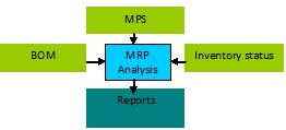
addition of certain financial modules, as well as the extension of MPS to deal with the full range of tasks in master planning and the support of business planning in financial terms, it is realized that the resultant system offered an integrated approach (MRP II) to the management of manufacturing resources. Browne, J., Harhen, J. (1992) defined MRP II as an extension of MRP to support the integrated management of many of the functions of the manufacturing enterprise. The MRP structure for relevant information is briefly summarized in figure 2.1.

Figure 2.1 MRP structure

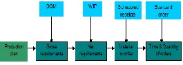
MRP analysis requires the input of BOM, MPS and accurate inventory status as shown in figure 2.1. On using MRP there are critical areas that include data accuracy, user know- how and system integrity to consider. The MRP process is as given in figure 2.2.

Figure 2.2 MRP process

MRP assumes that the MPS being fed into it is feasible in that adequate capacity exists to meet the requirements where an MPS is the plan that a company has developed for the production. It checks on the vendor and the manufacturing capacity beforehand. It sets the quantities of each end item to be produced in a given period, normally broken down into weekly targets of a short-range planning horizon.
MRP has the following weaknesses.
 Eliminates capacity planning

IJSER © 2012 http://www.ijser.org

International Journal of Scientific & Engineering Research, Volume 3, Issue 11, November-2012 3

ISSN 2229-5518

 Leave out task scheduling
 Use of inaccurate data is costly
 Quality MRP software is expensive
 Continuous training and development of
workers is costly
 Loss of inventory status data by accident distorts MRP operations
Running an MRP system can bring the following benefits.
 Reduced inventory levels
 Reduced component shortages
 Improved shipping performances
 Improved customer service
 Improved productivity
 Improved production schedules

2.1 The generic MRP model – [The case of

Gizmo-stools Inc.]

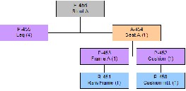
The starting point for MRP is BOM as shown in figure 2.3.

Figure 2.3 BOM for stool A

The BOM may have an arbitrary number of levels and will typically have purchased items at the bottom level of each branch in the hierarchy. The MRP system is based very simply on the fact that the BOM relationship allows one to derive the demand for component material based on the demand for the parent item.
The MRP system is driven by the MPS. Berry, W., Vollman, T. and Whybark, D. (1979) outlined that the MPS is derived from evaluating forecasts, customer orders, and distribution center requirements, which records the independent demand for top-level items. Table 2.1 below shows an order of 100
A-stools to be delivered 4 weeks from now.
Tables 2.2, 2.3, & 2.4 details the basic MRP
process by manual modeling.

Table 2.1 MPS for stool A

Current week is beginning of week one.

Table 2.2 MRP Calculations

Table 2.3 MRP Analysis for the stool A –

Extract of figure 2.3

IJSER © 2012 http://www.ijser.org

International Journal of Scientific & Engineering Research, Volume 3, Issue 11, November-2012 4

ISSN 2229-5518

Table 2.4 MRP Analyses for the ‘stool A’ Leg

- Extract of figure 2.3

Table 2.5 MRP Analyses for the ‘stool A’ Seat

– Extract of figure 2.3

3.0 HOW DOES MRP WORK?

In MRP, time is assumed to be discrete Berry, W., Vollman, T. and Whybark, D. (1979). Time is typically represented as a series of one-week intervals, though systems, which operate on daily planning periods, are readily available. Level codes are used, which refer to the lowest level of any BOM on which the component is to be found. Lead-time is standardized in
weeks. The lot sizing policy is defined, e.g., lot
for lot (L), by which the net requirement quantity is scheduled as the batch size for the replenishment order.

4.0 TOP-DOWN PLANNING WITH MRP

Top-Down planning considers ‘change’ as a continuous phenomenon, thus following the Kaizen approach. The MPS changes and the inventory status changes too. Four aspects of Top-Down planning are:
- Regenerative planning and net change,
- The frequency of Top-Down planning,
- The use of low-level coding
- Rescheduling in Top-Down planning.

4.1 Regenerative planning and Net change

Regenerative: Starts with the MPS and totally re-explodes it down through all the bills of materials to generative valid priorities. Net requirements and planned orders are completely generated at that time. The entire regenerative process is carried out in a batch- processing mode on the computer and, for all but the simplest of MPS, involves extensive data processing. Because of this, regenerative systems are typically operated in weekly and occasionally monthly re-planning cycles.

Net change: The MRP is continuously stored in the computer. Whenever there is an unplanned event, such as a new order in the MPS, an order being completed late or early, scrap or loss of inventory or engineering changes to the BOM, a partial explosion is initiated only for those parts affected by the change. If an event is planned, e.g., when an order is completed on time, then the original material plan should still be valid. The system is updated to reflect the new status but re- planning is not initiated.

Net change can operate in two ways. One mode is to have an on-line Net change system by which the system reacts instantaneously to unplanned changes as they occur. In most cases, however, change transactions are batched, by day, and re-planning happens

IJSER © 2012 http://www.ijser.org

International Journal of Scientific & Engineering Research, Volume 3, Issue 11, November-2012 5

ISSN 2229-5518

overnight. In the regenerative approach, there
is vulnerability because of the need to maintain the validity of the requirements plan between system-driven re-planning runs. The difference between the two is as follows [13]. Regenerative systems view the MPS as a document, new editions of which are released on a periodic basis. Net change systems see the MPS as a document, in a state of continuous change. The MPS is processed in terms of the changes, which have taken place since the last run.

4.2 The frequency of Top-Down planning

As we have seen, regenerative systems are typically re-planned on a weekly or monthly basis. Net change systems support more frequent re-planning, either on-line or batched in daily or weekly increments. There is a trade- off between data processing costs and the maintenance of valid priorities on manufacturing and purchase orders. The consensus view seems to be that the re- planning cycle should be no longer than a week.

4.3 The use of low-level coding

Low-level codes determine the sequence in which the processing of part requirements is carried out. Components may be common to many BOM product structures. In regenerative systems, if MRP processing were simply to follow a path through the BOM hierarchies in its re-planning it would, as a result, re-plan common components several times over. Low level coding is data processing mechanism, which saves to overcome this inefficiency.
The procedure is to assign to each component a code, which designates the lowest leveling on any BOM it is found. MRP processing then can proceed level by level and a component will not be planned until the level currently being processed is that of its low level code. Low-level codes are also a useful feature in net change systems when these systems are operated on a batch basis.

4.4 Rescheduling in Top-Down planning

Resolving production scheduling is difficult. When an MRP system is re-planning in a top- down fashion, it will typically adjust either the due date or the quantity of any planed order. If it identifies the need to make a change to an open order (a scheduled receipt), it typically sends an exception message for the materials planner to execute the change.
There is need to reschedule existing planned orders because of modifications to the MPS, or because of failure of a vendor or shop to deliver in the planned lead time or, indeed, any unplanned event. Rescheduling may involve the retiming of a planned order, as in the previous example, or it may require the modification of the order size or perhaps both. This is a trivial example and the solution presents itself readily.

5.0 BOTTOM-UP PLANNING WITH MRP

As pointed out earlier, an MRP system must react to change. In top-down planning, the system itself does the planning. An alternative is for the planner to manage the re-planning process. This is termed bottom-up re-planning and makes use of two tools as stated by Weiss, H., Gershon, M. (1992): the pegged requirements’ report and the firm planned order – both of which are described in this section.

5.1 Pegged requirements

Pegging allows the user to identify the sources of demand for a particular component’s gross requirements. The procedure of identifying each gross requirement with its source at the next immediate higher level in the BOM is termed single level pegging. Through a series of single level pegging reports, we can eventually trace a set of requirements back to their sources in the MPS. An alternative facility is full pegging where each individual requirement for a planned item is identified against a master production scheduled item and/or a customer order. This is a rare case. If

IJSER © 2012 http://www.ijser.org

International Journal of Scientific & Engineering Research, Volume 3, Issue 11, November-2012 6

ISSN 2229-5518

a lot sizing technique is used, it becomes
practically impossible to associate individual batches or lots with particular orders.

5.2 Firm planned order

The firm planned order allows the materials planners to force the MRP system to plan in a particular way, thus overriding lot size or lead time rules. A firm planned order differs from an ordinary planned order in that the MRP explosion procedure will not change it in any way. This technique can aid planners working with MRP systems to respond to specific material and capacity problems. A typical problem might be the failure of a vendor or the manufacturing plant to deliver an order within the allocated lead-time.
Assuming an MPS requirement for 100 of stool
A in week 10, this leads to plan availability of
100 of seat A by the end of week 8, and 100 each of frame A and the cushion by the end of week 7. Also, one can plan the availability of
400 of the legs at the end of week 8. The

unexpected occurs! It is informed that responsible manufacturing department cannot deliver the required amount of seat A until week 9 – one week late.

6.0 TIME REPRESENTATION IN MRP SYSTEMS

Bucketed systems limit the time horizon that may be considered and the granularity of timing that may be ascribed to an order. Bucket-less system enables daily visibility to an order’s date of requirement.

6.1 Bucketed and bucket-less MRP systems

In the bucketed approach, a predetermined number of data cells are reserved to accumulate quantity information by period. This is illustrated by the matrix structure used in the calculations of requirements. These data cells are known as time-buckets. A weekly time bucket contains all of the relevant planning data for an entire week. Since the number of buckets is predetermined, this means that there is a bound on the planning
horizon, depending on what time divisions the
buckets represent.
Weekly time buckets are considered to be the granularity necessary for near and medium term planning by MRP, whereas monthly buckets are considered too coarse. However, the normal bucket of one week may itself be too coarse to facilitate detailed short term planning. Further out in the planning horizon, monthly or perhaps quarterly time buckets are acceptable. There is no reason why the MRP system cannot accommodate a various time bucket size over the span of the planning horizon. In the non-bucketed approach each element of time phased data has a specific time label associated with it and is not accumulated into buckets. Consequently, the bucket-less approach is more flexible.

6.2 The planning horizon

The planning horizon refers to the span of time from the current date out to some future date, over which material plans are generated the chief factor in determining the planning horizon is the longest cumulative manufacturing and procurement time for a master scheduled item. The planning horizon is often extended further than the longest cumulative lead-time for the purpose of gaining visibility of manufacturing capacity needs in the future. The longer the planning horizon, the more difficult it is to make useful forecasts about the marketplace and the likely demand for products and end level items. The need to put in place an MPS over this planning horizon is the chief vulnerability of MRP systems. As Burbidge et al, (1985) says, “… It is not given to man to tell the future. …” A naïve reliance on a dubious MPS is a recipe for failure.

7.0 THE ROLE OF SAFETY STOCKS IN AN MRP SYSTEM

DeGarmo, E. P., J T. Black, and R. A. Kohser, (1997) describe safety stocks as quantities of stock that are to be maintained in inventory, to protect against unexpected fluctuations in

IJSER © 2012 http://www.ijser.org

International Journal of Scientific & Engineering Research, Volume 3, Issue 11, November-2012 7

ISSN 2229-5518

demand and/or supply. In this sense, safety stocks can be considered as insurance policy to cover unexpected events, whether such events are the failure of a vendor to meet a promised delivery date or an unexpected increase in demand for the product. However, given the high cost of tying up capital in inventory, the use of safety stocks can be expensive. Safety stocks can be incorporated into the MRP analysis. An alternative method is by subtracting the safety stocks from the initial inventory and then calculating the item net requirements in the usual way. The meaning of the projected inventory has changed and now refers to the projected physical stock less allocation, less safety stock.

8.0 THE CURRENT MRP STATE OF PRACTICE

Among the criteria that measure effective use of MRP are the following:
 MRP should use planning buckets no larger than a week
 The frequency of re-planning should be
weekly or more frequent
 If people are effectively using the system to plan, then the shortage list should have been eliminated.
 Delivery performance is 95 % or better for
vendors, the manufacturing shop, and
MPS.
 Performance in at least two of the following three business goals has improved: inventory, productivity, and customer service.
The various surveys taken through the years indicate the following several problems within MRP system implementations:
 Only very small % of users of MRP considers themselves to be successfully operating their MRP systems. Many systems are installed, as opposed to implementation, i.e., the formal system is not the real system.
 MPS is not computerized by MRP users as often as might be expected.
 CRP has a relatively low utilization by
MRP users.
 In relatively few cases is computerized
PAC implemented.

8.1 Reasons for failure of MRP installations

 Lack of top management commitment to the project
 Lack of education in MRP for those who will have to use the system
 Unrealistic MPS
 Inaccurate data
 Unpredictable order receiving trends
 Unrealistic price changes of raw materials in a competitive market

8.2 MRP in large corporations

Most large corporations that since implemented MRP have extended to MRP II approach system. This is consequently because MRP success was discovered to be so by management integration of many enterprise functions. Functional departments of a large corporation may classify as a cluster of relative SMEs. Large corporations aiming at maintaining a feedback loop system also commonly practice closed-loop MRP. This is afforded by combining the planning (MPS, MRP, and CRP) and execution modules (PAC and Purchasing) with the potential for feedback from the execution cycle to the planning cycle. Equally, ERP has recently emerged and is finding good use in these large corporations (Watson E. L., Medeiros D. J., Sadowski R. P., 1997, pp765).

8.3 MRP in SME manufacturing companies

An SME manufacturing company is characterized by few functions that are controllable. This makes MRP implementation easier though the assumption of adequate capacity requirements may be dwindled in some SMEs. However, following the current technological advancement leading MRP extension to MRP II, it has been a standing barrier for SMEs to afford implementation. MRP II is naturally impossible to start with in an SME setup because it is designed to support

IJSER © 2012 http://www.ijser.org

International Journal of Scientific & Engineering Research, Volume 3, Issue 11, November-2012 8

ISSN 2229-5518

the integrated management of many of the
functions of the manufacturing enterprise.

9.0 MANUAL & COMPUTERIZED MANIPULATION OF MRP DATA

Since 1980, the number of MRP installations increased. Manual and macro-computer models have been developed for different large corporations. These installations became available at lower cost on minicomputers and microcomputers. Some MRP computer programs activate other computer programs that perform other applications. Sales ordering, invoicing, billing, purchasing, production scheduling, capacity planning, and warehouse management are a few examples. [13] Today there is some concern as to how systems of the style of MRP can be integrated into a CIM environment and the adequacy of such systems compared with alternative philosophies such as Kan-ban/JIT and proprietary techniques such as OPT. [1]
The strength of manual manipulation is an economic one. It is a mathematical treatment of simple addition and subtraction using paper and pen. Starters without a computer can thus afford MRP at minimum overhead cost. A central strength of MRP computer program is its timely and accurate re-planning capability [13]. Various MRP software have been designed Vis-à-vis MRP plus, MRP21, MRP demo_version, MRP factory, ERP plus, SAP, SAGE and MRP Excel. The simplest of them all being MRP Excel that uses spreadsheets and visual basic database applications. The rest have been developed in MS Access database.

10.0 LOT SIZING IN MRP SYSTEMS

Lot sizing is from an economic perspective. For purchased items, vendors may supply only in multiples of a given number and the net requirements may have to be batched so as to accommodate this. A representative selection of the policy procedures will be reviewed that include: The lot for lot method, The fixed order quantity method, The economic order quantity method, The method
of fixed order periods, The periodic order
quantity method, The method of part period balancing and The Wagner Whitin algorithm. Other lot sizing methods, such as the Gaither method (1981), the modified Gaither method (1983), the Silver Meal technique (1973), or the method proposed by Groff (1979) was not looked into for reasons of their complexity especially considering the application to an SME setup.

10.1 The Lot for Lot method

It involves the direct translation of net requirements into order quantities. For each net requirement in each period there is an order offset by the appropriate lead-time.

10.2 The fixed order quantity method

This is frequently used. The net requirements are checked against the assigned fixed lot size. If the net requirements were less than or equal to the lot size, then the amount specified in the lot size is ordered. Otherwise the order size is equal to the net requirements.

10.3 The economic order quantity method

There is a setup cost incurred with the placing of an order or the start-up of a batch on a machine. This setup cost (for manufacturing items) or ordering cost (for purchased items) must be amortized over the batch or order size. There is a trade-off between order or setup costs and inventory costs. The economic order quantity (EOQ) formula is simply a mathematical expression of this trade-off and reflects the minimum total cost of carrying stock and setup.
EOQ = √ {2SD/C}
Where S = setup cost per batch, C = inventory carrying cost per item per unit time, Q = the batch size (EOQ), D = the demand for the item per unit time, TC = the total cost of inventory and setup; assuming that:
 Demand for the item in question is known and constant

IJSER © 2012 http://www.ijser.org

International Journal of Scientific & Engineering Research, Volume 3, Issue 11, November-2012 9

ISSN 2229-5518

 The setup cost and the inventory carrying cost are known

10.4 The method of fixed order periods

The method is similar to the fixed quantity method in the sense that it sets a fixed time between orders and orders the amount required to meet the demand in that period. The order period can be set on ad hoc basis or, perhaps, calculated on a similar basis to the EOQ described above to define a POQ that follows in the next section.

10.5 The periodic order quantity method

This is a variation of the fixed order period method where the ideas from EOQ are used to calculate the time between orders. This leads to variable order sizes with a fixed and constant time interval between orders. The time between orders is calculated by dividing the demand per period by the EOQ.

10.6 The method of part period balancing

The technique, as described by Berry (1972) and DeMatteis and Mendoza (1968), seeks to equate the cost of setup/order placement with the cost of inventory. It is based on the observation that the sum of the setup/ordering costs and the inventory costs in the EOQ formula are minimized at the point at which the two costs are equal.

10.7 The Wagner Whitin algorithm

This algorithm uses a dynamic programming approach to determine the optimum order quantities, given that the level of demand for a defined planning horizon is known and can be broken down into the discrete time periods and that the setup and the inventory carrying costs are known. It is dynamic in the sense that it deals with demand that varies over a discrete horizon and generates variable lot sizes economically to satisfy that demand.

11.0 FORECASTED INVENTORY STATUS

OF LE’S SAMPLE PRODUCTS

Two ranges of conveniently chosen final products were shown in table 11.1 below and their forecasted demand per week, as was technically sampled. These products are Mono pump’s Flex shaft Adaptor part- assembly and Conveyor Belt Fastener assembly, in all their various sizes. An inventory status is shown in table 11.2 for Flex shaft Adaptor part-assembly.

Table 11.1 Final Product forecast per week

Table 11.2 Flex shaft Adaptor part- assemblies inventory status

IJSER © 2012 http://www.ijser.org

International Journal of Scientific & Engineering Research, Volume 3, Issue 11, November-2012 10

ISSN 2229-5518

shown in figure 12.1. Thus, the order
enquiring procedure will follow a descriptive forecasted master production schedule.

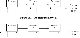
Figure 12.1 A JIT pull system

13.0 MRP SOFTWARE SPECIFICATION

An acceptance ranking criteria was conducted for modeling both manual & computerized MRP systems. Analysis results have shown that Computerized MRP system, Regenerative top-down planning, and bucketed time representation are best possible combinations for MRP use. Yet still the manual system though being least is most affordable by smallest entities without computers. Hence, two models were developed namely Manual MRP template & MRP Excel database as would be described herein under.

12.0 MRP DOMAIN EXPERTISE

LE’s order enquiring procedure follows typically a JIT system. It is definitely a pull
‘customer-driven’ system where production begins only when an order from the customer has been received. Information flows backwards as shown in figure 12.2. However, an MRP system changes LE‘s JIT pull-system domain into a push demand-driven system as
There is already designed MRP software on
the market. The researcher managed to come up with the following software tools merely applicable to manufacturing organizations. MRP plus is offered by Horizon software provider [19], which is designed in MS Access. MRP21 is offered by DBA software provider [20], and is designed in MS Access. MRP demo_version is offered by Merlin business software providers [21] and is designed in Visual Basic programming. MRP_DOS is offered by Weiss, J. H. (1992) programmable in MS DOS. MRP Excel version is offered by Tony Rice [18] and is designed in MS Excel.
However, following conclusion from a thorough selection criterion, MRP Excel version is highly favorable for SME organizations in Zimbabwe because of its simplicity, availability at minimum cost, flexibility, automation, user-interface and limitless data-entry capacity attributes.

13.1 Functional parameters

As for manual MRP manipulation (see form in Appendix 1), the parameters are basically the determination of the net requirements from the gross requirements after the BOM and inventory status. Following specified lead times; orders are planned and released as scheduled in set time-buckets and -horizons. In order to come up with a well-defined

IJSER © 2012 http://www.ijser.org

International Journal of Scientific & Engineering Research, Volume 3, Issue 11, November-2012 11

ISSN 2229-5518

systematic operation, manual MRP
manipulation-forms were designed.
Equally, Excel-based MRP system has the following domain features. VBA free, no macros, it is all formulae and PivotTables, and nothing is hidden. Demand is generated by a forecasted make-to-inventory Finite Schedule, but may also be from another source. A multiple level Bill of Material structure and inventory of raw material and components is allocated to the earliest scheduled product first, and will be dynamically re-allocated as the schedule changes. A Purchase Action Report identifies purchase orders which must be placed or chased to meet the schedule.
Then, the last spreadsheets of the system addresses an MRP question that many SME manufacturers have: "What products should I make with the inventory I have on hand right now?" The system takes into account raw materials that are used by more than one product, and ration the inventory across the products so as to even out the product inventory cover as much as possible.

13.2 Performance issues

The manual system realizes its weakness in performance because data cannot be quickly regenerated. The extra-mile that MRP Excel performs is to include the executable production schedule that is simply generated from rationalizing the purchase order report. Moreover, as was earlier derived, the MRP Excel must be a regenerative top-down planning system with bucketed time representation. The regenerative top-down MRP system manages data by itself once changes are fed in, which is impossible manually. Few spreadsheets are for data entry and the rest are regenerating directly or indirectly after clicking the refresh data icon. The system has a content page that links with every data spreadsheet and other important hyperlinks (HTM/HTML). Each spreadsheet links you back to the content page for quick access to other hidden sheets. It is, in addition, printable as a workbook for reporting
purposes or sharable through Local Area
Network and Electron Data Interchange systems.

14.0 DEVELOPMENT OF MRP SYSTEM MODEL FOR LE CO.

The MRP model shown in figures 14.1-4 was generated using the regenerative top-down planning system. For reasons of trading-off between re-planning costs and demand flow patterns, regeneration of data was minimized to one week. The bucketed time representation is in weeks. The time horizon exceeded LE Company‘s maximum lead-time of 6 weeks to arbitrarily 10 weeks.

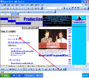
Click here to follow link

Figure 14.1 MRP excel front page

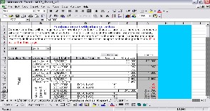
Figure 14.2 Purchase report with planned orders

IJSER © 2012 http://www.ijser.org

International Journal of Scientific & Engineering Research, Volume 3, Issue 11, November-2012 12

ISSN 2229-5518

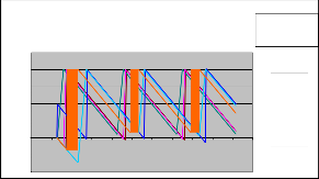
2.5

2.0

1.5

1.0

Projected Inventory

Cover

model. Otherwise, it was not going to reflect a
real-life small business setup. The same goes to all those who provided time and expertise when demanded without complain.

0.5

0.0

8-May 13-May 18-May 23-May 28-May 2-Jun 7-Jun 12-Jun 17-Jun 22-Jun 27-Jun 2-Jul

-0.5

-1.0

Figure 14.3 Projected Inventory Cover

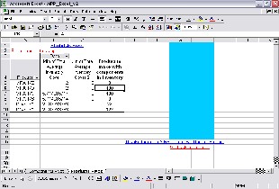
Figure 0.4 Products Pivot

15.0 CONCLUSIONS

The MRP Excel model developed was therefore recommended by the researcher for LE Company to deal with existing inventory planning and control problems. This Excel based MRP system model influenced a calculated minimum and acceptable payback period of 2 years & 1.7 months after investment for the analyzed products. Moreover it has much capacity to resist the unpredictable hyperinflation since it earns 37% as Internal Rate of Return at zero Net Present Value. Other SMEs manufacturers can use the same model and the researcher is available to assist them with data configuration and setup.

Acknowledgements

The researcher acknowledges the incessant effort put by the executive management team at Lane Engineering (LE) Company when they
openly shared useful data for generating this
Engineer Ngoni Chirinda is the current Director of Technology Centre at Harare Institute of Technology since 2009. Previously he served as acting chairperson of the department of Industrial & Manufacturing Engineering for one year. He also worked as a lecturer at the Harare Polytechnic College for 3 years in the Mechanical Engineering department. He received B Tech and M Sc degrees in Production Engineering and Manufacturing Systems & Operations Management respectively from the University of Zimbabwe. His research interests include factory automation systems and advanced manufacturing technologies. He is a registered professional engineer with the Engineering Council of Zimbabwe and is a member of the Zimbabwe Institute of Engineers.

REFERENCES

1. Ahmadian, A., Afifi, R., Chandler, W. (1990), “Readings in Production and Operations Management: A productivity perspective,” Allyn & Bacon, Boston, MA.
2. AICS, (1987), APICS Dictionary, 6th ed. American Production and Inventory control Society, Falls Church, VA, USA.
3. Berry, W. (1972), “Lot sizing techniques for requirements planning systems: a framework for analysis,” Production and Inventory management, 13(2), pp. 19-34.
4. Berry, W., Vollman, T. and Whybark, D.
(1979), “Master Production Scheduling, Principles and Practice,” American Production and Inventory control Society, Washington DC, USA.
5. Browne, J., Harhen, J. (1992), “Production
Management Systems,” 2nd ed., American Production and Inventory control Society, Washington DC, USA.

IJSER © 2012 http://www.ijser.org

International Journal of Scientific & Engineering Research, Volume 3, Issue 11, November-2012 13

ISSN 2229-5518

6. Burbidge, J. (1985), “Automated
Production Control with a simulation capacity”, in Modeling Production Management Systems, edited by P. Faister and R. Mazumber, Elsevier Science Publishers, pp.
19-35, Amsterdam, North-Holland.
7. DeGarmo, E. P., J T. Black, and R. A. Kohser, (1997), “Materials and Processes in Manufacturing”, 8th ed., Prentice-Hall, Englewood Cliffs, NJ.
8. Gono, G., (2006). “Fiscal policy statement,” in The Herald Newspaper, Herald Publishing Company, pp. 9, Harare, ZW. (publication date:
01/12/06)
9. Gupta, K. S., Zanakis, S. H., Mandakovic, T., (1990), “Software for production and operations management,”
Order # H16595.
10. Wagner, H. M., Whitin, T. M. (1958),
“Dynamic version of the economic lot size model”, Management Science, 5(1), pp. 89-96.
11. Heizer, I., Render, B. (1996), “Production and Operations Management,” Prentice Hall, New Jersey, USA.
12. Landers, T. L., Brown W. D., Fant E. W.,
Malstrom E. M., and Schmitt N. M. (1994), “Electronics Manufacturing Processes”, Prentice-Hall, Englewood Cliffs, NJ.
13. Orlicky J. (1975), “Material Requirements
Planning: The New Way of Life in Production
and Inventory Management”, McGrow-Hill,
New York.
14. Swearingen, J. “Integrated Manufacturing Planning and Control Systems,” PowerPoint lecture presentation: Penny State University.
15. Watson E. L., Medeiros D. J., Sadowski R. P. (1997), “A simulation-based backward planning approach for order release”, proceedings of the 1997 winter simulation conference, pp. 765.
16. Harhen, J. (1988), “The state of the Art of MRP/MRP II”, in “Computer Aided Production Management” edited by Rolstadas A., Springer Verlag, German.
17. Weiss, J. H., 1992. “PC: Software for production and operations management,” Order # H22916 [IBM 3 ½” version], Order # H22924 [IBM 5 ¼” version].
18. www.CNet.com/MRP_DOS/htm (date
accessed: 08/03/07)
19. www.DBAsoftware.com/mrp21_freeware

_demo./htm (date accessed: 15/03/07)

20. www.merlin_softwares.com/factoryMRP/ ERP_internetshop/htm (date accessed:

01/03/07)
21. www.mrppluss.com/fdownload_software/

httm (date accessed: 27/02/07)

22. www.production_scheduling.com/mrp_ex cel/htm (date accessed: 20/03/07)

IJSER © 2012 http://www.ijser.org

International Journal of Scientific & Engineering Research, Volume 3, Issue 11, November-2012 14

ISSN 2229-5518

APPENDIX

Appendix 1: Model 1 – MRP Worksheet/template

(Insert Company Logo) LE Company (Pvt.) Ltd

MRP Policy: ……………………

IJSER © 2012 http://www.ijser.org