International Journal of Scientific & Engineering Research, Volume 4, Issue 12, December-2013 65
ISSN 2229-5518
The Effect of Features Number on
Extended Observation-Cooperative SLAM
Gayas Asaad, Alireza Babaei, Mohammad H. Ferdowsi, Hossein Bolandi
Abstract— This paper investigates the effect of the number of environment features on a cooperative approach of simultaneous localization and mapping (SLAM). The tested cooperative SLAM approach is the Extended Observation-Cooperative SLAM (EO-CSLAM) algorithm which depends on additional, indirect correlated observations of the features (landmarks). The performance gain due to additional correlated observations means that additional features will have similar positive effect. However, as EO-CSLAM adopts extended Kalman filter-simultaneous localization and mapping (EKF-SLAM) solution, the number of environment features will have an important role in the computational burden. Simulation results show that the performance gain provided by EO-CSLAM is more obvious in tha less features cases.
Index Terms— Autonomous Navigation, Cooperative SLAM, Unmanned Surface Vehicles.
—————————— ——————————
hatever the task of an autonomous vehicle is, the accurate localization has an essential role for efficient achievement
and accurate results. For instance, in underwater environmental modelling, accurate navigation is very important to provide sensors with referential transformations matrix and high-accuracy
tween the local submaps, while the non-common features do not contribute to the improvement due to the uncorrelated nature of local submaps.
Consequently, in the case of absence of common features in the overlapped areas, which isa possible situation in large-
IJSER
pose [1]. On the other hand, while GPS can be used for
localization, its data can be inaccurate or inaccessible due to many possible reasons, such as atmospheric changes, noisy environments, multi-path errors, deliberate jamming, spoofing or confined areas where observing sufficient number of satellites can be difficult [2]. To solve these problems, simultaneous localization and mapping (SLAM) framework can be a proper alternative or incorporated to GPS [3]. Moreover, exploiting SLAM in a cooperative approach can provide more improvement in localization accuracy of USVs, in addition to the mentioned advantages of cooperative manners.
For the cooperative SLAM implementation with USVs, a Multi-USV-based CSLAM approach has been proposed in [5] using laser sensors. The research adopted the Constrained Local Submap Filter (CLSF) approach, which had been presented in [6] and [7] to improve computational efficiency and data association. In CLSF approach, local submaps are fused periodically into a single global map; the common (duplicated) feature estimates are processed by a constraining operation as a weighted projection to produce a recovered estimate for each common feature. Therefore, in theCLSF- based cooperative SLAM, the performance gain (versus the single-USV case) depends only on the common features be-
————————————————
• Dr. Alireza Babaei, Department of Aerospace, Amirkabir University of
Technology, Iran. E-mail: arbabaei@aut.ac.ir
• Dr. Mohammad H. Ferdowsi, Department of Electrical Engineering, Malek
ashtar University of Technology, Iran. E-mail: ferdowsi@mut.ac.ir
• Dr. Hossein Bolandi, School of Electrical Engineering, Iran University of
Science and Technology. . E-mail: h_bolandi@iust.ac.ir
scale environments, there will not be improvement in localiza-
tion accuracy and mappingperformance, and CLSF-based
CSLAM will act the same level of accuracy of Mono-SLAM or
lower.
In our previous work [8], the Extended Observation-
Cooperative SLAM (EO-CSLAM) has been presented, this
approach allows vehicles to improve localization accuracy and
mapping performance even with no common features, profit-
ing from all observed features, which makes it a proper meth- od for USVs using radar sensors.
In this paper more investigation on this algorithm is pre- sented showing the effect of environment features number on the resulting performance gain and computational complexity.
This paper is organized as follows: Section 2 provides the
general framework for the EO-CSLAM approach and its formulation, while section 3 evaluates (using simulations) the effect of features number on the performance gain and compu- tational burden. Finally, conclusions are presented in section 4.
In the general framework for the EO-CSLAM algorithm, it is assumed that a team of vehicles perform a collective task in an unknown environment. While moving through the environment, the vehicles use their sensors to obtain relative observations (measurements) of the features and vehicles within their fields of view (FOV). Assuming that the collaborating vehicles have the ability to share required information, each vehicle shares its observations and control signals with the collaborating vehicles.
For the marine environments case considered in this paper,
the collaborating vehicles are a team of USVs with radar
IJSER © 2013 http://www.ijser.org
International Journal of Scientific & Engineering Research, Volume 4, Issue 12, December-2013 66
ISSN 2229-5518
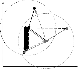
sensors. To demonstrate the algorithm, let’s consider the case of two USVs denoted a and b as shown pictorially in Fig.1
involving only three features for simplifying. The features on
updated values, for k = 1,2,3...
Prediction:
sea surface can be artificial and/or naturally occurring
sˆ a − =
(sˆ a + , ua ,0)
(2)
elements [4], [5].Considering the surface planar motion, the
start points of vehicles are firstly stored as initial positions
k f k − k −
with respect to a single global reference frame (XOY). Each
a − =
pk −1
ppk −1
pk −1
a +T
k −1
aT
k −1
k −1
pk −1
a +
pMk −1
(3)
vehicle initializes its global map in this frame with zero initial position uncertainty and then, continues (through the
where a
a
unknown environment) observing the features and vehicles in
Fpk −1 and L k −1 are the Jacobeans of motion model [9]:
its FOV. The relative observations and control data are shared between the vehicles; the shared features' observations are
As control data u v
b−
are shared, and having ( sˆ b+ ,
b−
b+
k −1
), the
used with the vehicle-vehicle (v-v) observations to generate
vehicle a obtains sˆ k
and Ck
of b using (2) and (3), so the v-
additional correlated observations, such as
z ab = z a + z b in
v observation a
1 b 1
Fig.1, while the shared control data are used by each USV to
zb is distinguished via data association (being
assigned to qˆ b − of sˆ b− ), and the shared local observations z v
k k ik
estimate and update the second vehicle's location. The
additional correlated observations are called extended observations (EO). Next subsection explains the details of the EO-CSLAM algorithm.
are used to obtain extended observations. See [8] for more details.
For all these types of observation, data association is performed: for each observation associated with previous
mapped feature, the innovationν a
and its covariance Eik are
FOV of a
Y f2
computed as follows:
For local observations z a :
IJSER
a a a ˆ a
a (ˆ a − , ˆ a )
z2 ν ik = zik − zik = zik − h sk mk
ba
2
(4a)
ab a
a − aT
a
Eik = Hik Ck
Hik
+ R k
(5a)
ab zb b
b f1
1
For extended observations z ab :
a ab
ˆ ab
ab (ˆ a − , ˆ a )
a ba
0 0
ν ik = zik − zik
= zik − h sk mk
(4b)
b a a − aT e
f0 z0
Eik = H ik Ck
H ik
+ R ik
(5b)
FOV of b
where H a![]()
= ∂h ∂s is the Jacobean of the observation model h :
O X a
![]()
![]()
∂h ∂h
Fig. 1: EO-CSLAM by two USVs (a, b), solid arrows refer to local observations (of features in the FOV) while dashed arrows refer to
extended observations, such as ab .
Hik = 01
∂p pˆ a −
Kalman gain:
.. 0i −1
∂f ˆ a ik
0i +1
.. 0 Nak
(6)
z1 a =
a − aT −1
K ik
Ck Hik Eik
(7)
2.1 EO-CSLAM algorithm formulation
The main quantities and their used symbols are defined in [8]
Update:
a + a − a a
together with way of obtaining extened observations.
sˆ k
= sˆ k
+ K ik ν ik
(8)
Therefore, it is enough (for this paper’s goal) to review the
a + =
a − − a
vT =
− a a a −
main EKF recursive procedure.
Ck Ck
K ik Eik K ik
(I K ik Hik )Ck
(9)
Initialization:
sˆ a + = pˆ a + = [ xˆ a + , yˆ a + , φˆa + ]T
(1)
while for each observation belongs to a new observed feature,
the location estimate fˆ a is computed as follows:
0 0 0 0 0
− xˆ a− + r
.cos(φˆa− + θ )
with covariance
Ca + = Ca +
, where no features have been
fˆ a
= g (pˆ k
, zik ) = k ik
k ik a −
(10)
0 pp0
ik
yk
+ rik .sin(φˆ
+ θik )
mapped yet ( ma = ∅). The vehicle a stores the initial data of
T a ab
both vehicles, i.e. ( sˆ a+ , Ca + ) and ( sˆ b+ , Cb + ). In the following,
where zik = [rik ,θik ]
represents zik or zik , and then, the new
0 0 0 0
a a− a −
the notation (⋅) − refers to predicted values, while (⋅) +
refers to
estimate is combined to
mˆ k
within
sˆ k
, while Ck is
k k
IJSER © 2013 http://www.ijser.org
International Journal of Scientific & Engineering Research, Volume 4, Issue 12, December-2013 67
ISSN 2229-5518
augmented, thus
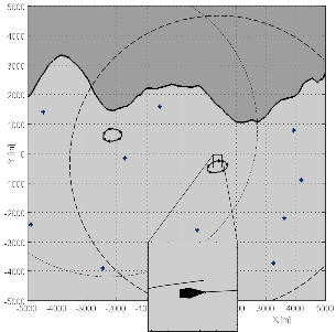
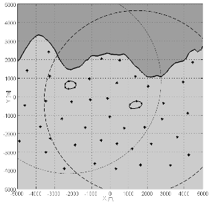
designed a simple virtual marine environment so that allows inserting point features and pre-planned trajectories to be fol-
a+ [
a− T
aT ˆ aT ]T
lowed by the USVs. Fig. 2 shows an example of
sˆ k
= (pˆ k )
Ca −
, mˆ k
Ca −
, fik
(J a Ca −
)T
(11a)
a 10km × 10km area with an arbitrary coast line and ten
ppk
pMk
p ppk
inserted features. The point features are assumed to be
Ca + = Ca − T
Ca −
(J a Ca −
)T
(11b)
outputs of signal processing algorithms [3] and extraction
k pMk
J a Ca −
MMk
J a Ca −
p pMk
Ca +
routines that detect the point targets while suppress land
p
where
ppk
p pMk
iik
a
reflections [4]. Two USVs ( a and b ) were inserted and driv- en along two closed trajectories of about 1.7 km-long. Dashed circles show the range/field-of-view FOV of each vehicle at
J a =
∂g![]()
∂pa
1 0
=
0 1
− rik .sin(φk
r .cos(φ a
+ θik )
+ θik )
(12)
the start time. The 5km-range of radar sensor was chosen
agreeing with actual detection capability on the sea surface
such as in [4].
and
a +
iik
is computed for local observations using R k :
a + a a − aT a aT
(13a)
Ciik
= J p C ppk J p
+ J z R k J z
and using R e
for extended observations
a + a a − aT
a e aT
(13b)
Ciik = J p C ppk J p
where
+ J z R ik J z
a
a a
a ∂g
cos(φk
+ θik )
− rik .sin(φk
+ θik ) b
J z =
= a
a (14)
∂zik
sin(φk
+ θik )
rik .cos(φk
+ θik )
and so, the next period ( k + 1 ) starts with (2) and (3)
continuing with the same manner.
2.2 Computational complexity
It has been mentioned that the Constrained Local Submap Filter (CLSF), which is an effective method for reducing the computational burden in small-scale environment, will not be useful for USVs with long-range sensors such as radar where the difference between the local and global map will be small. Therefore, among the methods used for reducing the compu- tational burden of SLAM algorithms, the state augmentation technique has been adopted in the EO-CSLAM algorithm, see (8) and (11 a,b); this technique reduces both the EKF predic- tion step and the process of adding new feature from calcula- tions with cubic complexity in the number of features to calcu- lations that are linear [10]. However, due the decentralized manner of EO-CSLAM and performing the SLAM procedure in each vehicle for additional observations increases the com- putational complexity of the algorithm. Section 3 compares the computational burden of EO-CSLAM with that of Mono- SLAM and illustrates the features’ number effect on the per- formance gain.
-200
-220
-240
-260
-280
-300
-320
1360 1380 1400 1420 1440 1460
Fig. 2: A simple marine environment including two USVs (a and b) on two closed trajectories (zooming in on b at the start point) with 10 features.
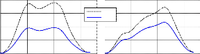
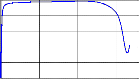
First, both Mono-SLAM and EO-CSLAM have been per- formed for the case of Fig 2, but with 6 features rather than 10. Considering the norm of positional error covariance as a total criterion for SLAM performance, Fig. 3 illustrates a comparison of norms of position covariance in both cases, Mono-SLAM and EO- CSLAM. It is obvious that the uncertainty in the vehicle position estimate via EO-CSLAM decreases noticeably versus Mono- SLAM. This improvement is due to the additional correlated fea- ture estimates generated by each vehicle through the extended observation way. Fig. 3 shows also the improvement ratio ( IR ) for each USV, which represents the reduction in the uncertainty as a percentage of the Mono case, defined as
This section demonstrates (using simulation) the positive role of additional features and observations on the localization accuracy using SLAM, in addition to their negative effect on computational burden, and how will be their role in the im- provement of EO-CSLAM approach.
In order to perform SLAM algorithm simulation, we have
|| Cqq ||Mono − || Cqq ||EO![]()
IR = × 100 %
|| Cqq ||Mono
(15)
IJSER © 2013 http://www.ijser.org
International Journal of Scientific & Engineering Research, Volume 4, Issue 12, December-2013 68
ISSN 2229-5518
the vehi cle a
8
6
4
Mono
EO
the vehi cle a
the vehi cle a
6
4
Mono
EO
the vehi cle a
2
2
0
50
40
30
20
10
0
0 500 1000 1500
Time [se c]
0 500 1000 1500
Time [se c]
0
50
40
30
20
10
0
0 500 1000 1500
Time [se c]
0 500 1000 1500
Time [se c]
Fig. 3: Comparison of two vehicles’ norm of covariance in Mono-SLAM
case with EO-CALM, and the improvement ratio for 6-Feature case.
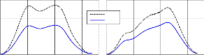
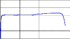
Next, the process has been repeated for 10-feature case and
40-feature case (Fig. 4). Fig. 5 illustrates the comparison for the
Fig. 5: Comparison of two vehicles’ norm of covariance in Mono-SLAM
case with EO-CALM, and the improvement ratio for 10-Feature case.
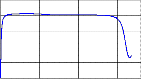
10-feature case, and Fig. 6 illustrates the 40-feature case. 3
Considering tha only the norm of vovariance and caomparing
it between the three cases (6, 10, and 40 features), it can be seen
that the increment in features number reduces the localization 1
errors for both, Mono-SLAM and EO-CSLAM, and despite that
EO-CSLAM is always better than Mono-SLAM, the performance 0
gain will be higher for the less features case; notice that the im-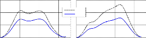
the vehi cle a
Mono
EO
the vehi cle a
IJSE30 R
provement ratio (IR) has reached 50% for the 6-feature case, while
for the 10- and 40-feature cases reached about 40% and 30%,
respectively. Furthermore, due to the correlation between the
vehicle postion eastimate and features locations estimates, the same effect and comparison will be satisfied for the mapping per-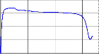
20
10
0
0 500 1000 1500
Time [se c]
0 500 1000 1500
Time [se c]
formance.
Fig. 6: Comparison of two vehicles’ norm of covariance in Mono-SLAM
case with EO-CALM, and the improvement ratio for 40-Feature case.
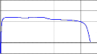
On the other hand, in the purpose of evaluating the computa- tional burden effect of the EO approach and its components, the running time elapsed (in MATLAB) for a single recursion period has been extracted for each method: Mono and EO-CSLAM.
a Fig. 7 shows this time for the vehicle b . As expected, the run-
b ning time increases in the cooperative approaches where a great- er amount of information is processed; while Mono-SLAM has the lowermost running time due to the least amount of shared
data, EO-CSLAM takes longest time. Thus, since the increment in processed data in SLAM increases the computational burden, more features means longer computating time for both Mono- SLAM and EO-CSLAM, and additionally, the longer computat- ing time is the price of the performance gain obtained using EO- CSLAM.
Fig. 4: The same marine environment case with 40 features.
IJSER © 2013 http://www.ijser.org
International Journal of Scientific & Engineering Research, Volume 4, Issue 12, December-2013 69
ISSN 2229-5518
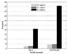
Fig. 7: Running time elapsed (in MATLAB) for a single recursion period for the 10 features’ case and vehicle b .
This paper has explaind the role of features number in the
REFERENCES
[1] H. Ferreira, C. Almeida, A. Martins, J. Almeida, A. Dias, G. Silva, E.
Silva “Environmental modeling with precision navigation using ROAZ autonomous surface vehicle,” in Proc. IROS – Intelligent Robots and Systems, Workshop on Robotics for Environmental Monitoring, Porto, Portugal, 2012.
[2] J. C. Leedekerken, M. F. Fallon and J. J. Leonard. “Mapping Complex
Marine Environments with Autonomous Surface Craft”, Massachu-
setts Institute of Technology, 77 Massachusetts Avenue, Cambridge,
MA 02139, 2010.
[3] G. Dissanayake, P. Newman, S. Clark, H.F. Durrant-Whyte, and M.
Csorba. “A solution to the simultaneous localisation and map build- ing (SLAM) problem,” IEEE Trans. Robotics and Automation,
17(3):229-241, 2001H. Poor, “A Hypertext History of Multiuser Di- mensions,” MUD History, http://www.ccs.neu.edu/home/pb/mud- history.html. 1986. (URL link *include year)
[4] J. Mullane, S. Keller, A. Rao, M. Adams, A. Yeo, F. Hover‡ and N.
Patrikalakis. “X-band Radar based SLAM in Singapore’s Off-shore,”
in Proc. IEEE, Int. Conf. Control, Automation, Robotics and Vision,
2010, pp. 398-403.
[5] M. Moratuwage, W. S. Wijesoma,B. Kalyan, J. Dong,and P. Namal
Senarathne. “Collaborative Multi-Vehicle Localization and Mapping in Marine Environments”, in Proc IEEE, Oceans’10, 2010.
[6] S.B. Williams. “Efficient Solutions to Autonomous Mapping and
IJSER
performance gain of the extended observation-cooperative SLAM
(EO-CSLAM). This role appears in two contradictory effects, a positive effect on the localization accuracy and mapping performaence (more features cause more accuracy for both Mono and EO-CSLAM), while the negative effect is the computational burden which incresea with the number of observed feature. While EO-CSLAM is always better than Mono-SLAM, the performance gain will be higher for the cases with less number of environment features.
Navigation Problems”, PhD thesis, University of Sydney, Australian
Centre for Field Robotics, 2001.
[7] S.B. Williams, G Dissanayake, and H Durrant-Whyte. “An Efficient
Approach to the Simultaneous Localisation and Mapping Problem”,
IEEE Proceedings. ICRA'02- Robotics and Automation, 2002.
[8] G. Asaad, A. Babaei, M. H. Ferdowsi, H. Bolandi, “Extended Obser-
vation-Cooperative SLAM for Unmanned Surface Vehicles.” Interna- tional Journal of Scientific & Engineering Research (IJSER), Vol. 4, Is- sue 8, (pp. 792–800) August 2013.
[9] Dan Simon, Optimal State Estimation, John Wiley & Sons, Inc., Ho-
boken, New Jersey, 2006. pp. 407-409.
[10] T. Bailey and H. Durrant-Whyte. “Simultaneous localization and mapping (SLAM): Part II, state of the art”, IEEE Robotics and Auto- mation Magazine 13(3), 108-117, 2006
IJSER © 2013 http://www.ijser.org