International Journal of Scientific & Engineering Research, Volume 3, Issue 10, October-2012 1
ISSN 2229-5518
I. I. Okonkwo, P. I. Obi , G. C Chidolue, S. S. N. Okeke
Abstract— State variable are crucial to transient simulation initialization of the electrical circuits. Other variable that are mathematically related to state variable may also be used to initialize transient response especially in symbolic simulation. In this paper we formulated and simulated electrical circuit transient symbolically using the transient nodal equation derived from branch effective current source. The result of the simulation agreed with the existing Matlab simpowersystem tool.
Index Terms— transient simulation, state variable, symbolic simulation, transient nodal equation, transient response, and electrical circuits.
—————————— ——————————
ome of the tasks that cannot be solved effectively by conventional simulation have become tractable by extending the simulation to operate a in symbolic domain. Symbolic
simulation involves introducing an expanded set of signal values
and redefining the basic simulation functions to operate over this expanded set. This enables the simulator evaluate a range of operating conditions in a single run. By linearizing the circuits with lumped parameters at particular operating points and attempting only frequency domain analysis, the program can represent signal values as rational functions in the s ( continuous time ) or z (discrete time) domain and are generated as sums of the products of symbols which specify the parameters of circuits elements [2 –
4]. Symbolic formulation grows exponentially with circuit size and it limits the maximum analyzable circuit size and also makes more difficult, formula interpretation and its use in design automation application [5 – 10]. This is usually improved by using semisymbolic formulation, which is symbolic formulation with numerical equivalent of symbolic coefficient. Other methods of simplification include simplification before generation (SBG), simplification during generation SDG, and simplification after generation (SAG) [11 – 17].
Symbolic response formulation of electrical circuit may be classified broadly as modified nodal analysis (MNA) [18], sparse tableau formulation and state variable formulation. The state variable method was developed before the modified nodal analysis, it involves intensive mathematical process and has major limitation in the formulation of circuit equations. Some of the limitations arise because the state variables are capacitor voltages and inductor currents [19]. The tableau formulation
G. C Chidolue and S. S. N. Okeke are Professors in Dept. Of
Electrical Engineering, Anambra State University, Uli. Nigeria.
has a problem that the resulting matrices are always quite large and the sparse matrix solver is needed. Unfortunately, the structure of the matrix is such that coding these routine are complicated. MNA despite the fact that its formulated network equation is smaller than tableau method, it still has a problem of formulating matrices that are larger than that which would have been obtained by pure nodal formulation [20]. In this paper a new nodal analytical method which is structured for easy simulation is introduced.
In this paper a nodal analytical method is introduced which may be used on linear or linearized RLC circuit and can be computer applicable and user friendly. The simplicity of the new transient nodal formulation lies in the fact that minimal node index is enough to formulate transient equation (1). Also standard method of building steady state nodal admittance bus is just needed to build the s – domain admittance bus while the branch source current are modified to its branch effective transient source current which comprises of the vector sum of the actual source current, its s – domain equivalent and the corresponding s – domain branch storage element induced current source due to transient inception (2). When these are done a complete transient nodal circuit equation can easily be formulated. In this paper, this new method is called s – domain nodal method of branch effective current source. Simplicity, compactness and economical is the advantage of the newly formulated mesh equation.
————————————————
Okonkwo and P. I. Obi are P. G. Scholars, in Dept. Of Elect.
Engineering, Anambra State University, Uli. Nigeria.
Y( s )V( s ) Je ( s )
where
Je ( s ) J( s ) JI ( s )
1
2
where also Y(s) is the Auxiliary admittance bus, s – domain
equivalent of nodal admittance, Je(s) is the transient nodal
IJSER © 2012
International Journal of Scientific & Engineering Research, Volume 3, Issue 10, October-2012 2
ISSN 2229-5518
equivalent current source, J(s) is the actual steady state nodal current source vector transformed to s – domain, and Ei(s) is the transient branch sum dc induced source current mesh vector at the instant of transient inception due to the constitutive sum
substituting equation (6) in (5) and simplifying to get
effect of branch storage elements on dc current flowing in these
respective branches around various meshes at that instant of
transient..
In this analysis branch companion model for R L C is
i4 (s) [V1(s) E4 (s) V2 (s)]Y4 (s) E(I)4 (s)Y4 (s)
i4 (s) [V1(s) V2 (s)]Y4 (s) E(e)4 (s)Y4 (s) i4 (s) [V1(s) V2 (s)]Y4 (s) J(e)4 (s) where
E(I)4 (s) i4 (0)Z(C)4 (s)
7
8
9
derived using laplace transform and then a generalized s- domain nodal equation is configured which is essentially
Z(C)4
(s) [L4
![]()
1 ]
ss1C4
modeled with a modified source current, modification and
derivation are follow
E(e)4
(s) E4
(s) E
(I)4
(s)
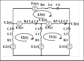
consider a three node circuit in fig 1, the generalization of nodal analysis of n th node may be demonstrated by forming equations of Kirchhoff’s current law at the three various
.
similarly i1
J(e)4 (s) E(e)4 (s)Y4 (s)
10
nodes, thus
i (s) V (s)Y (s) J
(s)
11
1 1 1
(e)1
For Node 2
similarly i5
i5 (s) [V1(s) V3 (s)]Y5 (s) J(e)5 (s) 12
The sum of the current flowing onto node 1 may be obtained by adding equation (9), (11) and (12) to get
V1 (s)[Y1 (s) Y4 (s) Y5 (s)] V2 (s)Y4 (s) V3 (s)Y5 (s)
J(e)1 (s) J(e)4 (s) J(e)5 (s)
13
For Node 2
Similarly, the Kirchhoff ’s current equation for node 2 may be written as follows
V2 (s)[Y2 (s) Y4 (s) Y2 (s)] V1 (s)Y4 (s) V3 (s)Y6 (s)
J(e)2 (s) J(e)4 (s) J(e)6 (s)
14
Figure 1: Three Nodes, Three Mesh Rlc Electrical Circuit.
For Node 3
Similarly, the Kirchhoff ’s current equation for node 3
may be written as follows
V3 (s)[Y3 (s) Y5 (s) Y6 (s)] V1 (s)Y5 (s) V2 (s)Y6 (s)
i1 i4 i5 0
3
J(e)3 (s) J(e)5 (s) J(e)6 (s)
15
For i4
equations (13), (14)and (15) are combined to get the nodal equation for fig 1 circuit as follows
The constitutive effect of the branch elements is as follows
Y ( s )
Y ( s )
Y ( s ) V ( s ) J
( s )
d 1 11 12
13 1
( eN )1 ![]()
![]()
V1(t) E4 (t) V2 (t) R4 (t) L4 dt i (t) c
i4 (t)
4
Y21( s )
Y22 ( s )
Y23 ( s )V2 ( s ) J( eN )2 ( s )
16
4 Y
( s ) Y
( s ) Y
( s )V ( s ) J
( s )
taking the laplace transform of equation (4)
31 32
33 3
( eN )3
V1 (s) E4 (s) V2 (s)
Y11 (s) Y1 (s) Y4 (s) Y5 (s)
Y (s) Y (s) Y (s) Y (s)
[R
sL
1 ]i
(s) L i
(0) VC4 (0)
5
22 2 4 6
![]()
4 4
4
but![]()
4 4 s
Y33 (s) Y3 (s) Y5 (s) Y6 (s) Y12 ( s ) Y21 ( s ) Y4 ( s )
17
VC4
![]()
(0) i4 (0)
s1C4
6
Y13 (s) Y31 (s) Y5 (s)
Y23 ( s ) Y32 ( s ) Y6 ( s )
IJSER © 2012
International Journal of Scientific & Engineering Research, Volume 3, Issue 10, October-2012 3
ISSN 2229-5518
J(eN)1 J(e)1 (s) J(e)4 (s) J(e)5 (s) J(eN)2 J(e)2 (s) J(e)4 (s) J(e)6 (s) J(eN)3 J(e)3 (s) J(e)5 (s) J(e)6 (s)
18
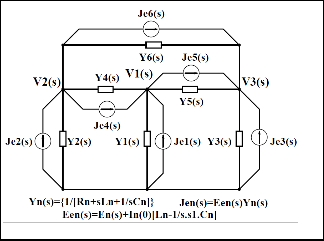
method of building an admittance bus so far the branch admittances Yk(s) of the circuit are evaluated as in equation (25). In this paper it is called the s – domain auxiliary impedance bus.
also
V (s)
J (s)
NODAL EQUATION
V(s)
V2 (s) ,
J (s)
Je 2
(s)
,
28
Equation (16) may be used to generalize the nodal solutions
e
n – th node in laplace frequency domain when all the branch
Vm (s)
Je m (s)
effective source currents have been formulated as follows.
V(s) and Je(s) are the vector of nodal transient voltage and
Y (s)
Y12 (s)
Y1n (s) V1 (s)
(eN)1
transient nodal effective current source respectively, all in
Y21(s)
Y22 (s)
Y2n (s) V2 (s) J(eN)2 (s)
19
frequency domain.
Yn1(s)
Yn2 (s)
Ynn (s) Vn (s)
J(eN)n (s)
K
J(eN)n (s) J(e)k (s)
k 1
K
J(e)k (s) [Ek (s) Ik (0)Z(C)k (s)]Yk (s)
k 1
K
J(e)k (s) [Ek (s) E(I)k (s)]Yk (s)
k 1
18
19
20
Z(C)k
(s) [Lk
![]()
1 ], ss1Ck
s1 jω
21
E(e)k (s) Ek (s) E(I)k (s)
where
E(I)k (s) Ik (0)Z(C)k (s)
J(e)k (s) E(e)k (s)Yk (s)
22
23
24
Fig 2: S – Domain Nodal Equivalent Diagram.
Yk (s)
Rk
![]()
1
sLk
![]()
1 sCk
25
k=1, 2- - - (K – th) branch that are incident on (n – th) node n=1, 2 -
- - (N – th).
Ik(0) → is the dc current flowing in the (k – th) branch at the
The generalized compact form of the equation (19) is thus as follows
instant of transient.
Ek (s) → is the Laplace transform of the source voltage in the (k –
th) branch.
Z(C)k(s) → is the net transfer impedance for the transient dc
quantities in the frequency domain due to the energy
where
V(s)Y(s) Je(s)
26
storing components in the (k – th) branch Z(C)k(s) transforms the dc current Ik(0) flowing in (k – th) branch to transient dc source voltage E(I)k(s) in that branch.
E(I)k(s) → is the transient dc induced source voltage in the (k – th)
branch at the instant of transient inception due to the
Y (s)
Y12 (s)
Y1n (s)
constitutive effect of the branch transient impedance
Y(s)
Y21 (s)
Y22 (s)
Y2n (s)
27
operator Z
(s) on the dc current I (0) flowing in that
(C)k k
branch at that instant.
E (s) → is the effective source voltage in the (k – th) branch due
Yn1 (s)
Yn2 (s)
Ynn (s)
(e)k
to the net effect of source voltage and the induced dc
Y(s) is laplace frequency domain admittance bus, the admittance could be built from fig 2 using any standard
source voltage during transient in frequency domain.7
J(e)k(s) → is the effective source current in the (k – th) branch ource
IJSER © 2012
International Journal of Scientific & Engineering Research, Volume 3, Issue 10, October-2012 4
ISSN 2229-5518
current during transient in frequency domain.
J(e)n(s) → is the sum of the effective source in all the (k – th)
branches incident ondue to the net effect of source
current and the induced dc s the (n – th) node.
1. Calculate the steady state branch current.
2. Transform all the branch admittances to their s – domain
equivalents.
3. transform all the branch voltage sources to their s –
method(use laplace transformation.
4. Calculate the branch dc driving point impedance
Z(c)k(s),equation (10b)and use equation (10c) to calculate the branch dc induced branch source voltage.
5. Use equation (10c) to calculate equivalent transient current source.
6. Draw the s – domain equivalent of the RLC circuit by replacing the steady state circuit admittances with their s domain equivalents as they are calculated in step two. Also replace the branch steady state source current with their branch transient equivalent source current as calculated in step five.
7. From the s – domain transient equivalent circuit
diagram, use any of the steady state method of
formulating nodal equation to formulate s – domain
transient nodal equation. It is worthy to note that
formulated s – domain equivalent circuit is structurally a
mere corollary of steady state circuit diagram. This is also true between the formulated transient nodal
equation and the steady state mesh equation.
8. Form equation (16) and solve for V(s) using Cramer’s
rule.
9. Transform V(s) to time domain equivalent using laplace
inverse transform. Eg. in Matlab,
Generator 2
E2(t)=0.8|E1|sin(t+450), ZG2=(4+j36), S=1MVA Line Parameters
Rs=0.075 /km, Ls=0.04875 H/km Gs=3.75*10-8 mho/km, Cs=8.0x10⁻⁹F/km Line length=100 km, Fault position = 60%
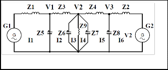
A single pi section was adopted as a model for the test circuit. Normally the model is characterized with constant parameter, shunt capacitance of transmission line is included in the analysis while shunt conductance is neglected. The equivalent circuit of the test circuit is below fig 4.
Fig 4: Single line equivalent circuit (PI model) for earth faulted transmission line.
In this paper the transient nodal voltages were simulated by using the described formulation (s – domain nodal equation by method of branch effective transient current source). Analysis procedures of section 3 were used to calculate the s – domain
V( t ) ilap(V( s ))
23
rational functions of the nodal voltages (19). The obtained s –
domain rational functions were transformed to close form
from this nodal voltages could easily be obtained at any
instant.
An earth faulted 100 kV - double end fed 100 km single transmission line was used for verification of the formulated s – domain transient nodal equation. In this analysis fault position is assumed to be 60%.
continuous time functions using laplace inverse transformation. Discretizations of the close form continuous time functions were done to obtain to plot the nodal voltage response graphs.
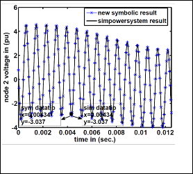
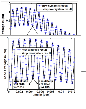
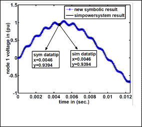
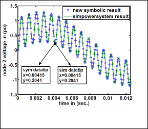
To validate the formulated transient nodal equation, a simulation of the earth faulted double end fed, single transmission line were also performed using Matlab simpowersystem software to obtain the circuit transient nodal voltage responses. Results were compared with the responses obtained from the symbolic simulations using the formulated transient nodal equation.
Fig 3: Earth faulted Single line
Test Circuit Parameters
Generator 1
E1(t)=10x104sin(t), ZG1=(6+j40), S=1MVA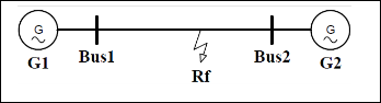
Nodal voltage response were simulated using the formulated nodal equation and also using simpowersystem package, all simulation were done using Matlab 7.40 mathematical tool. Simulated responses by these methods for the earth faulted
IJSER © 2012
International Journal of Scientific & Engineering Research, Volume 3, Issue 10, October-2012 5
ISSN 2229-5518
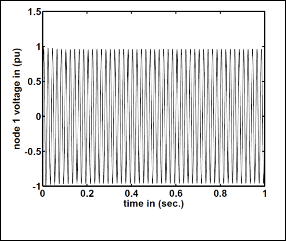
double end fed single line transmission were obtained and shown in fig 5 through fig 12. Possible data taking point of node 1and node 3 were taken for various simulating conditions. Simulating conditions included; zero initial condition, non – zero initial condition, high resistive (1000) fault but at zero initial condition, and 1 sec. simulation. All simulations were done, except otherwise stated on 100km line at 60% fault position and 5 earth resistive fault. Sampling interval for the formulated equation simulation is 50 S while that of the simpowersystem simulation is at 5 S. The overall result showed almost 100% conformity between new nodal symbolic formulation and the simpowersystem simulation.
100 km Line, Fault Position=60% and 5 Resistive Earth Fault.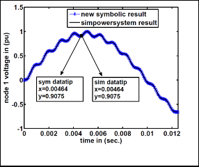
.
Fig 4: Simulation of Nodal Voltages Versus
Time; 0% Initial Condition.
.
Fig 7: Simulation of Nodal Voltages versus Time; Initial Conditions, 0.033 Sec of Steady State Run
.
Fig 8: Simulation of Nodal Voltages versus Time;
0% Initial Condition, and 1000
Resistive Earth Fault.
IJSER © 2012
Fig 6: Simulation of Nodal Voltages versus Time; Initial Conditions, 0.033 Sec of Steady
State Run
International Journal of Scientific & Engineering Research, Volume 3, Issue 10, October-2012 6
ISSN 2229-5518
Simulation software has been formulated for transient simulation of RLC circuits initiated from steady state. The simulation software is especially useful for power circuits that are modeled with Pi – sections parameter. The result of the simulation of this new symbolic nodal software showed promising conformity with the existing simpowersystem package and has the advantage of being able to simulate imaginary initial conditions. Structurally the formulated nodal equation can easily be modified to simulate subtransient response of RLC circuits.
Fig 9: Simulation of Nodal Voltages versusTime;
0% Initial Condition, and 1000 Resistive
Earth Fault.
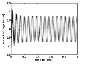
Fig 10: Simulation of Nodal Voltages versus; 0% Initial Condition. Earth Fault
Fig 11: Simulation of Nodal Voltages versus;
0% Initial Condition.
[1] Randal E. Bryant” Symbolic Simulation—Techniques And Applications”. Computer Science Department, Paper 240. (1990)
[2] C.-J. Richard Shi And Xiang-Dong Tan “Compact Representation And Efficient Generation of S-Expanded Symbolic Network Functions For computer-Aided Analog Circuit Design” IEEE Transactions On Computer-Aided Design Of Integrated Circuits And Systems, Vol. 20, No. 7, July 2001
[3] F. V. Fernández, A.Rodríguez-Vázquez, J. L. Huertas, And G. Gielen, “Symbolic Formula Approximation,” In Symbolic Analysis Techniques: Applications To Analog Design Automation, Eds. Piscataway, NJ: IEEE, 1998, Ch. 6, Pp. 141–178.
[4] Gielen And W. Sansen, Symbolic Analysis For Automated Design Of Analog Integrated Circuits. Norwell, Ma: Kluwer, 1991.
[5] Mariano Galán, Ignacio García-Vargas, Francisco V.
Fernández And Angel Rodríguez-Vázquez “Comparison
Of Matroid Intersection Algorithms For Large Circuit
Analysis” Proc. Xi Design Of Integrated Circuits And
Systems Conf., Pp. 199-204 Sitges (Barcelona), November
1996.
[6] M. Galán, I. García-Vargas, F.V. Fernández And A.
Rodríguez-Vázquez “A New Matroid Intersection
Algorithm For Symbolic Large Circuit Analysis” Proc. 4th
Int. Workshop On Symbolic Methods And Applications To
Circuit Design, Leuven (Belgium), October 1996
[7] A. Rodríguez-Vázquez, F.V. Fernández, J.L. Huertas And G.
Gielen, “Symbolic Analysis Techniques And Applicaitons
To Analog Design Automation”, IEEE Press, 1996.
[8] M. A. Al-Taee, F. M. Al-Naima, And B. Z. Al-Jewad, “Symbolic Analyzer For Large Lumped And Distributed Networks”, Chapter 23 In The Book: Symbolic – Numeric Computations, Wang, Dongming, Zhi, Li-Hong (Eds.), Series: Trends In Mathematics, Pp. 375-394, Birkhauser Verlag Basel, Switzerland, Feb 2007.
[9] W. Chen And G. Shi, “Implementation Of A Symbolic Circuit Simulator For Topological Network Analysis,” In Proc. Asia Pacific Conference On Circuits And Systems (Apccas), Singapore, Dec. 2006.
IJSER © 2012
International Journal of Scientific & Engineering Research, Volume 3, Issue 10, October-2012 7
ISSN 2229-5518
[10] Z. Kolka, D. Biolek, V. Biolková, M. Horák, “Implementation Of Topological Circuit Reduction”. In Proc Of Apccas 2010, Malaysia, 2010. Pp. 951-954.
[11] Tan Xd, “Compact Representation And Efficient Generation Of S-Expanded Symbolic Network Functions For Computeraided Analog Circuit Design”. IEEE Transaction On Computer-Aided Design Of Integrated Circuits And Systems, 2001. P. 20
[12] Wambacq P, Gielen G, Sansen W, “A New Reliable Approximation Method For Expanded Symbolic Network Functions”. IEEE Int. Symposium On Circuits And Systems (Iscas). Atlanta, 1996.
[13] R. Sommer, T. Halfmann, And J. Broz, “Automated Behavioral Modeling And Analytical Model-Order Reduction By Application Of Symbolic Circuit Analysis For Multi-Physical Systems”, Simulation Modeling Practice And Theory, 16 Pp. 1024–1039. (2008).
[14] Q. Yu And C. Sechen, “A Unified Approach To The Approximate Symbolic Analysis Of Large Analog Integrated Circuits,” Ieee Trans. On Circuits And Systems – I: Fundamental Theory And Applications, Vol. 43, No. 8, Pp. 656–669, 1996.
[15] P. Wambacq, R. Fern´Andez, G. E. Gielen, W. Sansen, And A. Rodriguez- V´Zquez, “Efficient Symbolic Computation Of Approximated Small-Signal Characteristics,” IEEE J. Solid-State Circuit, Vol. 30, No. 3, Pp. 327–330, 1995.
[16] O. Guerra, E. Roca, F. V. Fern´Andez, And A. Rodr´Iguez- V´Azquez,, “Approximate Symbolic Analysis Of Hierarchically Decomposed Analog Circuits,” Analog Integrated Circuits And Signal Processing, Vol. 31, Pp. 131–
145, 2002.
[17] X. Wang and L. Hedrich, “An approach to topology synthesis of analog circuits using hierarchical blocks and symbolic analysis”, Proc. Asia South Pacific Design Automation Conference, Jan. 2006, pp. 700-705
[18] Ho Cw, Ruehli A, Brennan P., “The Modified Nodal Approach To Network Analysis”. IEEE Trans. Circuits Syst., P. 22. (1975)
[19] Ali Bekir Yildiz “Systematic Generation Of Network Functions For Linear Circuits Using Modified Nodal Approach” Scientific Research And Essays Vol. 6(4), Pp.
698-705, 18 February, 2011
[20] R. Sommer, D. Ammermann, And E. Hennig “More Efficient Algorithms For Symbolic Network Analysis: Supernodes And Reduced Analysis, Analog Integrated Circuits And Signal Processing 3, 73 – 83 (1993)
IJSER © 2012