International Journal of Scientific & Engineering Research, Volume 6, Issue 1, January-2015 618

ISSN 2229-5518

Support Vector Machine Classification using

Mahalanobis Distance Function

Ms. Hetal Bhavsar, Dr. Amit Ganatra

Abstract— Support Vector Machine (SVM) is a powerful technique for data classification. The SVM constructs an optimal separating hyper-plane as a decision surface, to divide the data points of different categories in the vector space. The Kernel functions are used to extend the concept of the optimal separating hyper-plane for the non-linearly separable cases so that the data can be linearly

separable. The different kernel functions have different characteristics and hence the performance of SVM is highly influenced by the selection of kernel functions. Thus, despite its good theoretical foundation, one of the critical problems of the SVM is the selection of the appropriate kernel function in order to guarantee high accuracy of the classifier. This paper presents the classification framework, that uses SVM in the training phase and Mahalanobolis distance in the testing phase, in order to design a classifier which has low impact of kernel function on the classification accuracy. The Mahalanobis distance is used to replace the optimal separating hyper- plane as the classification decision making function in SVM. The proposed approach is referred to as Euclidean Distance towards the Center (EDC_SVM). This is because the Mahalanobis distance from a point to the mean of the group is also called as Euclidean distance towards the center of data set. We have tested the performance of EDC_SVM on several datasets. The experimental results show that the accuracy of the EDC_SVM classifier to have a low impact on the implementation of kernel functions. The proposed approach also achieved the drastic reduction in the classification time, as the classification of a new data point depends only on the mean of Support Vectors (SVs) of each category.

Index Terms— Classification, Euclidean distance, Kernel function, Mahalanobis distance, optimal hyper-plane, Support Vector

Machine, Support Vectors

1 INTRODUCTION

——————————  ——————————
he classification is the task of assigning the class labels to data objects based on the relationship between the data items with a pre-defined class label. The classification techniques are helpful to learn a model from a set of training data and to classify a test data well into one of the classes. There are several well known classification algorithms like Decision Tree Induction, Bayesian Network, Neural Network, K-nearest neighbors and Support Vector Machine [1], [2], [3],
and [4].
SVM have attracted a great deal of attention in the last decade and have actively been applied to various domain applica- tions. SVMs are typically used for learning classification, re- gression or ranking function and have been shown to be more accurate as compared to other classification models. SVM are based on statistical learning theory and structural risk minimi- zation principal and have the aim of determining the location of decision boundaries also known as hyper-plane that pro- duce the optimal separation of classes [5], [6], [7]. It has been shown in [4] that the hyper-plane that optimally separates the data is obtained by minimizing the following function:

(1)
- al re ts n to d-

————————————————

• Hetal Bhavsar is currently pursuing Ph. D. in Computer Engineering at

Charusat University, Changa and working as a Assistant Professor in

Dept. of Computer Sci. & Engg., The M. S. Univeristy of Baroda, Vadoda-

ra, India. E-mail: het_bhavsar@yahoo.co.in

• Dr. Amit Ganatra, H. O. D., Computer Engineering Dept., Charusat Uni-

versity, Changa, India. E-mail: amitganatra.ce@charusat.ac.in

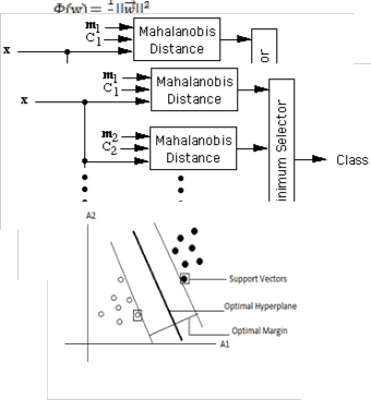
Fig. 1: Conventional SVM classifier with optimal separating hyper-plane and support vectors

SVM can also be extended to learn non-linear decision func-

IJSER © 2015 http://www.ijser.org

International Journal of Scientific & Engineering Research, Volume 6, Issue 1, January-2015 619

ISSN 2229-5518

tions. This can be done by first projecting the input data onto a high-dimensional feature space using kernel functions and formulating a linear classification problem in that feature space [6][7].
Using the kernel function, the optimization classification func- tion in the high dimensional feature space turns to be:

(2) The kernel function measures the similarity or distance be-

tween the two vectors. A kernel function K: is valid if there is some feature mapping, such that
(3) Thus, we can calculate the dot product of with-
out explicitly applying function to input vector. Here, we do not need to know how to map the sample information from original space to feature space [6], [7], [8].
Generally SVM models perform better classification tasks with very complex boundaries when data points are mapped into a high dimensional feature space using kernel functions. Some of the common well-performing kernel functions in most cases are [8], [9], [10] and [11]:

 Linear Kernel: k(xi , xj ) = xi · xj

 Polynomial Kernels: k(xi , xj)=(γ(xi , xj) + r)d , r ≥0, γ>0

 Radial Basis Function Kernels (RBF): k(xi , xj )=exp(-

||xi , xj ||2 / 22) where σ > 0

 Sigmoid Kernel: k(xi , xj) =tanh(α (xi , xj) + r), r ≥ 0

Each of these kernel functions has their own characteristics. For example, linear and polynomial kernel functi on has global characteristic, means samples far from each other can affect the val- ue of kernel function, while the RBF kernel functi on has local char- acteristic which onl y allows samples closed to each other to i nflu- ence the value of kernel functi on [12]. A sigmoid kernel function is similar to a two-layer perceptron neural network while RBF kernel is similar to RBF neural network [6]. In case of RBF ker- nel function the feature space is an infinite dimensional while in case of polynomial it is finite. Polynomial kernel function produces a polynomial separating hyper-plane whereas Gaussian RBF kernel function produces a Gaussian separating hyper-plane. So, depending on the level of non-separability of data set, the kernel function should be chosen. With an appro- priate selection and implementation of the kernel function in SVM, the trade-off between the classification complexity and classification error can be controlled.
Therefore, to obtain the optimal performance of the SVM clas- sification, it is necessary to select an appropriate kernel func- tion. This means, the SVM classification accuracy is highly dependent on the selection of kernel function. This is due to the fact that the separability of data points is different in fea- ture space of different kernel functions. Thus, one of the criti- cal problems of the SVM classification is the selection of ap- propriate kernel function, based on the type of datasets, in order to have high classification accuracy. It does not have generally an optimal kernel function which is able to guaran- tee good classification performance on all types of datasets of
varying characteristics. Also, each kernel function has parame- ters whose value has to be changed and tuned according to the data set. For instance as we change the value of the degree m in polynomial kernel function, we move from a lower dimen- sion to a higher dimension. In case of Gaussian kernel func- tion, ρ decides the spread of the Gaussian. Choosing the opti- mal values of these parameters is also very important along with the selection of kernel function. In recent years, many research works have been carried out in order to solve the problem of automatically finding the most appropriate kernel function and parameters for the SVM in order to guarantee high accuracy of the classifier.
In this work, an improved classification framework is pro- posed, which we call as EDC_SVM. It uses Mahalanobis dis- tance function to replace the optimal separating hyper-plane of the conventional SVM. The proposed framework first finds the support vectors of each category from the training data points and then the mean of support vectors of each category is calculated by mapping them into original vector space. During the classification phase, to classify a new data point, the distances between the new data point and the mean of support vectors of each category are calculated in the original vector space using the Mahalanobis distance function. The classification decision is then made based on the category of the mean of support vectors which has the lowest distance with the new data point, and this makes the classification de- cision irrespective of the efficacy of hyper-plane formed by applying the particular kernel function.

2 RELATED WORK

Selection of kernel function and the parameters of the kernel function is the critical problem of SVM classification since its evaluation. Grid search algorithms are used to find the best combination of the SVM kernel and parameters, but these al- gorithms are iterative and increase the computational cost of SVM during the training phase [13]. As a result, the efficiency of the SVM classifier has been severely degraded by having such methods in determining the appropriate combination of kernel and parameters. The evolutionary algorithm is pro- posed to optimize SVM parameters, including kernel type, kernel parameters and upper bound C, which is based on the genetic algorithm [14]. This is an iterative process by repeating the crossover, mutation and selection procedures to produce the optimal set of parameters. The convergence speed depends on the crossover, mutation and selection functions in evolu- tionary algorithm.
The method which avoids the iterative process of evaluating the performance for all the parameter combination is proposed in [15]. In this approach, the kernel parameter selection is done using the distance between two classes (DBTC) in the feature space.. The optimal parameters are approximated accurately with sigmoid function. The computation complexity decreases significantly since training SVM and the test with all parame- ters are avoided. Empirical comparisons demonstrated that the proposed method can choose the parameters precisely, and the computation time decreases dramatically.

IJSER © 2015 http://www.ijser.org

International Journal of Scientific & Engineering Research, Volume 6, Issue 1, January-2015 620

ISSN 2229-5518

A method using the inter-cluster distances in the feature spac- es to choose the kernel parameters for training the SVM mod- els is proposed in [16]. Calculating such distance costs much less computation time than training the corresponding SVM classifiers; thus the proper kernel parameters can be chosen much faster. With properly chosen distance indexes, the pro- posed method performs stable with different sample sizes of the same problem. As a result, the time complexity of calculat- ing the index is possible to be further reduced by the sub- sampling strategy in practical usage, and thus the proposed method can work even the data size is large. However, the penalty parameter C is not incorporated into the proposed strategies in which the training time of SVM might be further minimized.
Although very accurate, the speed of SVM classification de- creases with increase in the number of support vectors. The method of reducing the number of support vectors through the application of Kernel PCA is described in [17]. This meth- od is different from other proposed methods as the exact choice of the reduced support vectors is not important as long as the vectors span a fixed subspace. This method reduces the number of support vectors by up to 90% without any signifi- cant degradation in performance. The advantage of the meth- od is that it gives comparable reduction performance to other complicated methods based on quadratic programming and iterative kernel PCA.
A new feature weight learning method for SVM classification is introduced in [18]. The basic idea of the method is to tune the parameters of the Gaussian ARD kernel via optimization of kernel polarization, and each learned parameter indicates the relative importance of the corresponding feature. Experi- mental results on some real data sets showed that, this method leads to both an improvement of the classification accuracy and a reduction of the number of support vectors.
A new text classification framework is based on the Euclidean distance function, which have low impact on the implementa- tion of kernel function and soft margin parameter C is pre- sented in [19]. The classification accuracy of the Euclidean- SVM approach is relatively consistent with the implementa- tion of different kernel functions and different values of pa- rameter C, as compared to the conventional SVM. However, the classification phase of the Euclidean-SVM approach con- sumes a longer time as compared to the conventional SVM. Besides this, for certain classification tasks where the similari- ty between categories is high, the classification accuracy of the Euclidean-SVM approach is lower than the accuracy of con- ventional SVM approach. This is due to the fact that the Eu- clidean distance calculation which inherits the characteristic of nearest neighbor approach, may suffer from the curse of di- mensionality, hence leads to the inefficient classification tasks. In high dimensional space the data becomes sparse and tradi- tional indexing and algorithmic techniques fail from an effi- ciency and or effectiveness perspective. Aggarwal et al. [20] viewed the dimensionality curse from the point of view of the distance metrics which are used to measure the similarity be- tween the objects. They examine the behavior of the common- ly used Lk norm and showed that the problem of meaningful- ness in high dimensionality is sensitive to the value of k. They introduced fractional distance metrics as an extension of the
Lk norm, and showed that fractional distance metric provides more meaningful results from the theoretical and empirical perspective. The result of this research has powerful impact on particular choice on distance metric.
However, the choice of kernel function and parameter selec- tion is still complex and difficult. Therefore, the goal of this paper is to propose the new framework for SVM, which has low impact on the selection and implementation of kernel function and parameters of kernel function.

3 MAHALANOBIS DISTANCE FUNCTION

The Mahalanobis distance is mainly used in classification problems, where there are several groups and the investiga- tion concerns the affinities between groups. It is also used in pattern recognition or discriminant analysis, where the know- ing the mean of groups (m) and covariance matrix (, a new element (x) can be classified into one of these groups with as little chance of error as possible [21]. The Mahalanobis dis- tance is defined as:

(4) The Mahalanobis distance as a minimum-distance classifier

can be used as follows. Let m1 , m2 , …, mc be the means for the


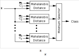
c classes, and let C1 , C2 , ... , Cc be the corresponding covari-
ance matrices. A feature vector can be classified by measur- ing the Mahalanobis distance from to each of the means, and assigning to the class for which the Mahalanobis distance is minimum as shown in Fig. 2.

Fig. 2: Assigning class label to a point x, using Mahalanobis distance

The use of the Mahalanobis metric as a distance measure is more advantageous compared to Euclidean distance measure, as it automatically accounts for the scaling of the coordinate axes, corrects for correlation between the different features, provides curved as well as linear decision boundaries and also works well for high dimensional data sets.
The Mahalanobis distance measure is also valid to use if the data for each class is similarly distributed. If the variables in x for each group were scaled so that they had unit variances, then C would be the identity matrix and in mathematical terms, the Mahalanobis distance is equal to the Euclidean dis- tance between the feature vector x and the group-mean vector m, which can also be referred as Euclidean distance towards the centre of data [22], [23]. We called this Euclidean distance

IJSER © 2015 http://www.ijser.org

International Journal of Scientific & Engineering Research, Volume 6, Issue 1, January-2015 621

ISSN 2229-5518

towards the center of data as EDC and it can be defined as,

(5) Since, the proposed research work uses scaled data, the varia- tion of Mahalanobis distance i.e. EDC, is used and so the pro- posed framework has been named as EDC_SVM.

4 EDC_SVM CLASSIFICATION FRAMEWORK

The proposed classification framework replaces the optimal separating hyper-plane of the conventional SVM by EDC dis- tance function as the classification decision making function. We still need to construct the optimal separating hyper-plane to recognize the SVs, in the training phase of EDC_SVM. This can be done by mapping the training data points into the fea- ture vector space and use the conventional SVM training algo- rithm to identify the SVs of each category.

After the SVs for each of the categories have been identified, they are mapped into the original vector space and mean of SVs of different categories are calculated. Once the mean of SVs of different categories are calculated, all the training data including SVs are eliminated. During the classification phase, a new unlabeled data point is mapped into the same original vector space, and the distances between the new data point and mean of SVs of each category are com- puted using the EDC dis- tance function and the lowest dis- tance is used to make the classification deci- sion.

Fig. 3: Vector space of EDC_SVM classifier with the EDC distance func- tion

Fig. 3 represents how the classification of the new unlabeled data point can be done using EDC_SVM. Let the hollow circles represents the SVs of category 1 and dark circles represents the SVs of category 2. As illustrated in Fig. 3, mean m1 and m2 is calculated for the support vectors of category 1 and 2, re- spectively. After obtaining the mean, the EDC distance be- tween the new data point represented by square and the mean m1 and m2 has been computed. The EDC distance of new data point to mean of SVs of each category is,
which has the lowest distance.
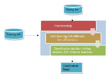
Fig. 4 illustrates the framework of the EDC_SVM classification approach.

Fig. 4: EDC_SVM classification frame work

EDC_SVM algorithm is illustrated as follow:
Pre-processing Phase
1. Transform all the data into numerical format, as SVM
works only on numerical data.
2. Libsvm framework is used for experimental purpose, so data need to be converted into format acceptable to Libsvm. It is represented as 1:1 3:2.
Training Phase
1. Map all the training data points into the vector space
of a SVM.
2. For each category, recognize and obtain the set of support vectors using SVM algorithm, and eliminate the rest of training data points which are not the sup- port vectors.
3. Calculate the means of SVs for each category by map-
ping them into original vector space.
4. Eliminate SVs also.
Testing Phase
1. Map new unlabeled data point into the same original
vector space.
2. Use EDC distance function to calculate the distance
between the new data point and the mean of each cat- egory.
3. Identify the category which has the lowest distance between its mean and the new data point.
4. The classification result is generated based on the
identified category for the new data point.

(6)

The classification decision is then made based on the category
By combining the SVM training algorithm and variation of the

IJSER © 2015 http://www.ijser.org

International Journal of Scientific & Engineering Research, Volume 6, Issue 1, January-2015 622

ISSN 2229-5518

Mahalanobis distance function, EDC, to make the classification decision, the impact of kernel function on the classification accuracy of the conventional SVM can be minimized. This is due to the fact that the transformation of existing vector space into a higher dimensional feature space by the kernel func- tions is not needed during the classification phase, as the sup- port vectors, mean of the support vectors and data points to be classified are mapped into the same original vector space, and hence do not have great impact on the classification perfor- mance. As a result, we can obtain an enhanced EDC_SVM classifier with the accuracy comparable to the conventional SVM, while unaffected from the problem of determining the appropriate kernel functions.
This approach also achieves drastic reduction in the classifica- tion time. In conventional SVM, to find the class label of new data point, it is required to evaluate the kernel function be- tween the new data point and each support vector. The num- ber of SVs can still increase with the number of data point and hence the classification time. On the other hand, in EDC_SVM, to find the class label of new data point, it is required to evalu- ate distance between a point and only the mean of SVs of each category, which depends only on the number of categories. Therefore, it takes very less classification time compared to the conventional SVM.

4.1 Complexity:

Let n be the number of training points, s be the number of SVs and c be the number of categories in the data set, and each feature vector x is of m dimensional.

Training time and space complexity:

Standard SVM training has O(n)3 time and O(n)2 space com- plexities. The SVM implementation used for the experiments is the Sequential Minimal Optimization (SMO) method, which is based on the concept of decomposition. The time complexity of SMO has been calculated empirically to O(n)2, while the space complexity will be reduced drastically, as no matrix computation is required.
Since, the EDC_SVM uses SMO in training phase, the training time complexity of EDC_SVM is O(n)2.

Classification time Complexity:

The classification time complexity of EDC_SVM is depends only on the point to be classified and the mean of SVs of each category. The mean of SVs of each category is already calcu- lated during the training phase. Since there are c categories, numbers of means are c.
So, the classification time complexity for classification of n new points is O (n * c), which leads the classification complexi- ty to O (n), as c<<n.

5 EXPERIMENTAL RESULTS

The proposed EDC_SVM classification framework has been tested and evaluated using four datasets of different character- istics. Datasets considered are of increasing dimensions and
also with increasing number of training and testing instances. Datasets available in this repository are collected from UCI and other very popular machine learning repository. This re- search considered iris, a1a (adult) and wine dataset from LIBSVM [24] and DNA dataset1.

5.1 Experimental Setup and Preliminaries:

The experiments have been conducted by implementing the conventional SVM classification approach and EDC_SVM in- dependently with four different kernel functions: Linear, Pol- ynomial, RBF and Sigmoid. Complexity or regularization pa- rameter C controls the trade-off between maximizing the mar- gin and minimizing the training error term, which is set to 1 for all experiments. All the kernel functions are run with the default parameters, such as, Polynomial kernel with degree d=3, RBF kernel with =1/number of features and Sigmoid kernel with =1/number of features. Parameter tuning is not required, as with these default parameters EDC_SVM gives best result. The simulation results for conventional SVM are taken by running SMO algorithm using LIBSVM framework. The EDC_SVM are implemented by using the same version of SMO and LIBSVM. Using the training module of SMO, the set of SVs of each of the categories are identified and then we have developed an additional module to calculate the EDC distance between the new data point and mean of set of SVs of each category. The measures like accuracy, number of correct- ly classified instances (CCI), precision, True Positive Rate (TPR) and False Positive Rate (FPR) are used to compare the performance of EDC_SVM with conventional SVM.

5.2 Experiments on IRIS data:

The very well known IRIS data set consists of 50 samples from each of three species of Iris (Iris setosa, Iris virginica and Iris versicolor). Four features were measured from each sample: the length and the width of the sepals and petals, in centime- ters. All three species of Iris are separable.
Table 1 show the experimental results of the conventional SVM and EDC_SVM classifier, which have been implemented with the different kernel functions and with the default values of parameters for iris dataset.
As illustrated in Table 1, the performance of the conventional SVM is highly dependent on the implementation of the kernel functions. The linear, RBF and sigmoid kernel have contribut- ed to high classification accuracies, which is 97%. On the other hand, the polynomial kernel has poor performance on iris dataset, with an accuracy of 75.33%. This result into high variance of accuracies (118.655) across the different kernel functions. This shows that the wrong implementation of ker- nel function leads to a poor performance of the SVM. In other words, the implementation of appropriate kernel is required to guarantee the good generalization ability for SVM classifier. As for the performance of EDC_SVM for on iris dataset, we have obtained classification accuracies between the range of

1 https://www.sgi.com/tech/mlc/db/

IJSER © 2015 http://www.ijser.org

International Journal of Scientific & Engineering Research, Volume 6, Issue 1, January-2015 623

ISSN 2229-5518

93.33% to 94.66% with the implementation of different kernels and default kernel parameters. Table 2 also shows that the EDC_SVM has around 3% less accuracy for linear, RBF and sigmoid compared to conventional SVM, but the average ac- curacy of EDC_SVM is higher than that of conventional SVM. The EDC_SVM also has very less variance (0.2948) among the
accuracies for different kernel functions compared to conven- tional SVM. Hence it has been concluded that EDC_SVM is unaffected from the implementation of kernel function in or- der to obtain the good classification accuracy.
Table 1: Result of Conventional SVM and EDC_SVM with different kernels, on IRIS dataset

Table 2: Result of Conventional SVM and EDC_SVM with different kernels, on Wine dataset

Table 1 also shows that the number of SVs is same for both the
approaches, but the classification time for EDC_SVM ap- proach is less compared to conventional SVM, as it needs only the mean of SVs of each category, instead of SVs, for classifica-
tion of new data point. Testing time of classification phase for both approaches with the different kernel implementation is shown in Fig. 5.

Fig. 5: Testing time for Conventional SVM and EDC_SVM for different kernels on IRIS dataset

5.3 Experiments on Wine Dataset

These data are the results of a chemical analysis of wines grown in the same region in Italy but derived from three different cultivars. The analysis determined 178 training sam- ples with the quantities of 13 constituents found in each of the three types of wines.

IJSER © 2015 http://www.ijser.org

International Journal of Scientific & Engineering Research, Volume 6, Issue 1, January-2015 624

ISSN 2229-5518

Table 2 shows the experimental results of the conventional SVM and EDC_SVM classifier, which have been implemented with the different kernel functions and with the default values of parameters for Wine dataset. As illustrated in Table 2, the performance of the conventional SVM with linear, RBF and sigmoid kernel have contributed to high classification accura- cies, which is 99% while with polynomial kernel has con- tributed to poor performance with an accuracy of 40.44%. This results into high value of variance of accuracies (859.357) for different kernel functions. This is due to the fact that, the wrong implementation of kernel function leads to a poor per- formance of the SVM.
On the other hand, the performance of different kernel func- tions with EDC_SVM on wine dataset is nearly consistent, with accuracy in the range of 91.01% to 96.06. This result into variation in accuracy for EDC_SVM is very less compared to conventional SVM as shown in Table 2. Though, the highest accuracy achieved by EDC_SVM is 3% less than the highest accuracy achieved by conventional SVM, but average accuracy of EDC_SVM is 9% more than SVM. Hence it has been con- cluded that EDC_SVM is unaffected from the implementation of kernel function in order to obtain the good classification accuracy.
Fig. 6 shows that the classification time is same for EDC_SVM with different kernel functions as it does not depend on the number of SVs.

Fig. 6: Testing time for Conventional SVM and EDC_SVM for different kernels on W ine dataset

5.4 Experiments on Adult Dataset

This dataset predict whether income exceeds $50K/yr based on census data, also known as "Census Income" dataset. The original Adult data set has 14 features, among which six are continuous and eight are categorical. In this data set, continu- ous features are discretized into quantiles, and each quantile is represented by a binary feature. Also, a categorical feature with m categories is converted to m binary features. Therefore, the final data set consists of 123 features. The dataset has 1605 training samples and 30956 testing samples.
Table 3 shows the experimental results of the conventional SVM and EDC_SVM classifier, which have been implemented with the different kernel functions and with the default values
of parameters for Adult dataset.
Based on the Table 3, it can be observed that the implementa- tion of the different kernel functions has affected the perfor- mance of the conventional SVM on Adult dataset. As ob- served, for the conventional SVM, the linear, RBF and sigmoid kernel have contributed to high classification accuracies, which is 83%. On the other hand, the polynomial kernel has poor performance on adult dataset, with an accuracy of
75.94%.
For Adult dataset, the performance of EDC_SVM is slightly affected by the implementation of kernel functions. The EDC_SVM has achieved high performance for polynomial, RBF and sigmoid kernel function with the consistent accura- cies of 83.55%, while it showed less performance on linear kernel function with an accuracy of 77.4%. This is due to the fact that, categories in adult data set are very similar to each other. Hence it is difficult to make them separable with linear kernel. Though there is slight affection of implementation of

kernel function in EDC_SVM, the average accuracy achieved by it is higher and the variance of accuracies among different kernel functions is lower than the conventional SVM, as shown in Table 3.
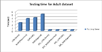
As the number of testing instances is more compared to train- ing instances, the testing time for conventional SVM is higher than the training time and it is also depends on the number of SVs. On the other hand both the times are nearly same in EDC_SVM, and classification time is order of 10 less than the conventional SVM, as the classification phase of EDC_SVM depends only on the mean of SVs of each category. The com- parison of classification time of is shown in Fig. 7.

Fig. 7: Testing time for Conventional SVM and EDC_SVM for different kernel, on Adult dataset

5.5 Experiments on DNA dataset

The problem posed in this dataset is to recognize, given a se- quence of DNA, the boundaries between exons (the parts of the DNA sequence retained after splicing) and introns (the parts of the DNA sequence that are spliced out). This problem consists of two subtasks: recognizing exon /intron boundaries (EI sites), and recognizing intron /exon boundaries (IE sites).

IJSER © 2015 http://www.ijser.org

International Journal of Scientific & Engineering Research, Volume 6, Issue 1, January-2015 625

ISSN 2229-5518

Three classes (neither, EI and IE) are there [21]. The data set has 2000 training data points and 1186 testing data points and each data points has 180 attributes.
Table 4 shows the experimental results of the conventional SVM and EDC_SVM classifier for DNA dataset. As illustrated inTable 4, for the conventional SVM, the linear, RBF and sig- moid kernel have contributed to high classification accuracies,
which is 94%. On the other hand, the polynomial kernel has poor performance on DNA dataset, with an accuracy of
50.84%. This result into the variance of 461.45 in the classifica- tion accuracies for different kernel functions. Based on
the result, it can be observed that the implementation of the different kernel functions has affected the performance of the conventional SVM on DNA dataset.
Table 3: Result of Conventional SVM and EDC_SVM with different kernels, on Adult dataset

Table 4: Result of Conventional SVM and EDC_SVM with different kernels, on DNA dataset
Fig.
8
also

sho ws that, as
On the other hand, the EDC_SVM is not dependent of the im- plementation of kernel functions. The EDC_SVM has achieved classification accuracies between the ranges of 88.76% to
90.72%, with the implementation of different kernels. This ac- curacy is slightly less than the highest accuracy obtained by conventional SVM, but the average accuracy of EDC_SVM is around 6% more than conventional SVM. The variance of ac- curacies among different kernel functions is (0.904) very less compared to conventional SVM. In other words, EDC_SVM has better consistency in terms of accuracy with the imple- mentation of different kernel function as compared to the con- ventional SVM classifier.
with the other data set, for the DNA data set also the classifi- cation time is reduced by order of 10, even though the num- bers of SVs are large. It can also be observed that it takes same time for all the kernel functions, as it depends on number of category and not on SVs.

IJSER © 2015 http://www.ijser.org

International Journal of Scientific & Engineering Research, Volume 6, Issue 1, January-2015 626

ISSN 2229-5518

[8] K. Muller, S. Mika, G. Ratsch, K. Tsuda, B. Scholkopf, “An Introduction to Ker- nel Based Learning Algorithms,” CRC Press, 2002. IEEE Transaction on Neural Networks Vol. 12, no. 2, pp. 181-201, 2001.

[9] R. Herbrich. Learning kernel classifiers: theory and algorithms. pp. 17-110, The

MIT press, 2002.

Fig. 8: Testing time for Conventional SVM and EDC_SVM for different kernel on DNA dataset

6 CONCLUSION

The proposed approach EDC_SVM has the following ad- vantages compared with the conventional SVM.
• The performance of the EDC_SVM classification has low dependency on the implementation of kernel functions.
• The accuracy of EDC_SVM is consistent with different kernel functions.
• There is a loss of accuracy compared to conventional SVM, but the average accuracy of EDC_SVM is higher than the conventional SVM.
• The classification time required by EDC_SVM is less as it required finding the distance between the new data point to be classified and the mean of the SVs of each category.
• The classification time taken by EDC_SVM is same for all the four kernel functions considered, no matter how many SVs are, as it depends only on the number of categories, which is same for all kernels.

REFERENCES

[1] J. Han and M. Kamber, Data Mining Concepts and Techniques, Elevier, 2011.

[2] S. B. Kotsiantis, “Supervised Machine Learning: A Review of Classification

Techniques,” Informatica, vol. 31, pp. 249-268, 2007.

[3] Thair N. Phyu, “Survey of Classification Techniques in Data Mining,” in Inter-

national Multiconference of Engineers and Computer Scientists, Hong

Kong, 2009.

[4] H. Bhavsar, A. Ganatra, “A Comparative Study of Training Algorithms for

Supervised Machine Learning”, International Journal of Soft Computing and Engineering (IJSCE) ISSN: 2231-2307, Volume-2, Issue-4, September

2012.

[5] A. M. Javier ,M. Moguerza, “Support Vector Machines with Applications,”

Statistical Science , vol. 21, no. 3, pp. 322-336, 2006.

[6] C. J. Burges, "A Tutorial on Support Vector Machines for Pattern Recognition," Data Mining and Knowledge Discovery, vol. 2, 1998.

[7] V. Vapnik, C. Cortes, “Support Vector Network,” Machine Learning, vol. 20, pp. 273-297, 1995.

[10] C. Campbell, and Y. Ying. "Learning with support vector machines."Synthesis

Lectures on Artificial Intelligence and Machine Learning 5.1, 1-95, 2011.

[11] B. Scholkopf and A. J. Smola. “ Learning with Kernels: Support Vector Ma- chines, Regularization, Optimization and Beyond. MIT press, 2002.

[12] H. Bhavsar and A. Ganatra. “Increasing Efficiency of Support Vector Machine using the Novel

Kernel Function: Combination of Polynomial and Radial Basis Function”, Interna-

tional Journal on Advanced Computer Theory and Engineering (IJACTE),

vol. 3, no. 5, pp. 17-24, 2014.

[13] C. Staelin. "Parameter selection for support vector machines." Hewlett-Packard

Company, Tech. Rep. HPL-2002-354R1, 2003

[14] A. T. Quang, Q. L. Zhang, and X. Li. "Evolving support vector machine param- eters." Machine Learning and Cybernetics, 2002. Proceedings. 2002 International Conference on. Vol. 1. IEEE, 2002.

[15] J. Sun. "Fast tuning of SVM kernel parameter using distance between two clas- ses." Intelligent System and Knowledge Engineering, 2008. ISKE 2008. 3rd Interna- tional Conference on. Vol. 1, pp. 108-113. IEEE, 2008.

[16] K. P. Wu, and S. D. Wang. "Choosing the kernel parameters for support vector machines by the inter-cluster distance in the feature space." Pattern Recognition 42, no. 5, pp. 710-717 , 2009.

[17] N. Sundaram. "Support vector machine approximation using kernel

PCA." Univ. California at Berkeley, Berkeley, CA, USA, Tech Rep. UCB/EECS-

2009-94.[Online]. Available: http://www. eecs. berkeley.

edu/Pubs/TechRpts/2009/EECS-2009-94. pdf , 2009.

[18] T. Wang. "Improving SVM classification by feature weight learning."Intelligent Computation Technology and Automation (ICICTA), 2010 International Confer- ence on. Vol. 2., pp. 518-521, IEEE, 2010.

[19] L. H. Lee, C. H. Wan, R. Rajkumar and D. Isa.. "An enhanced support vector machine classification framework by using Euclidean distance function for text document categorization." Applied Intelligence vol. 37, no.1, pp. 80-99, 2012.

[20] C. C. Aggarwal, A. Hinneburg, and D. A. Keim. On the surprising behavior of distance metrics in high dimensional space. Springer Berlin Heidelberg, pp. 420-434,

2001.

[21] G. J. McLachlan. "Mahalanobis distance." Resonance 4.6, pp. 20-26, 1999.

[22] S. Xiang, F. Nie, and C. Zhang. "Learning a Mahalanobis distance metric for

data clustering and classification." Pattern Recognition, vol. 41, no.12, pp. 3600-3612,

2008.

[23] R. De Maesschalck, D. Jouan-Rimbaud, and D. L. Massart. "The mahalanobis distance." Chemometrics and intelligent laboratory systems vol. 50, no.1, pp. 1-18,

2000.

[24] C. C. Chang, and C. J. Lin. "LIBSVM: a library for support vector ma- chines." ACM Transactions on Intelligent Systems and Technology (TIST), vol. 2, no.3, 27, 2011

IJSER © 2015 http://www.ijser.org