INTERNATIONAL JOURNAL OF SCIENTIFIC & ENGINEERING RESEARCH, VOLUME 4, ISSUE 1Ř, MBER-2013

ISSN 2229-5518

1373

Study of vertical distribution of tropospheric

Aerosol Number Density

Pratibha B. Mane

Abstract- Atmospheric aerosols are the suspension of fine particles in the Earth’s atmosphere. Aerosol measurements have been carried out at Kolhapur (16°42′N, 74°14′E) by using newly designed Semiautomatic Twilight Photometer. Some noticeable features of the semiautomatic twilight photometer are improvement in efficiency of the system, signal to noise ratio, height resolution, low level intensity measurement, duration of operation of the system, rate of sampling, accuracy in storing the data etc. The twilight scattering method yields a reasonable qualitative picture of the day-to-day variability of the vertical distribution of the aerosol number density per cm3 (AND) (Here after aerosol number density per cm3 is called as AND) from about 6 km to a maximum of 350 km. The tropospheric aerosol loading showed monthly and seasonal variations also. The monthly variations were in good agreements with Hindu lunar months. More sets of observations are essential to arrive at definite conclusion. The aerosol loading at 6-7 Km showed well agreement between morning and evening aerosol loading, (exceptions of cloudy period). The Lower middle tropospheric aerosol loading (at 6-7 Km) was ~10 times and ~15 times higher than that of middle and higher tropospheric aerosol loading respectively.

Keywords: aerosols, Twilight sound method (TSM), aerosol vertical distribution, Twilight Photometer, troposphere, Twilight Photometer, aerosol number density

——————————  ——————————

1. INTRODUCTION

aerosols. Kolhapur city, a location in the south-west
Maharashtra is selected for this study because this station is
Atmospheric aerosols are the suspension of fine particles in Earth‟s atmosphere. Depending upon the source size of aerosols varies from 10-3 to 102 μm. Particles larger than 100 μm cannot remain suspended in atmosphere for long periods. The examples of various forms of common aerosols are dust, smoke, mist, fog, haze and smog.
Twilight scattering method (TSM) is extensively used by
several workers in all over the world to study the vertical
distribution of atmospheric aerosol particles which is a
strong function of their sources, sinks and their residence
times. All this study is reviewed by Jadhav et al. [1] which
is mainly on the stratospheric aerosols. The tropospheric
aerosols are least studied. The Earth‟s atmosphere is
divided into five main layers. Starting from the Earth‟s surface these layers are named as: Troposphere (situated altitude between 0 and 17 kilometers), Stratosphere (between 17 and 50 kilometers), Mesosphere (located about
50 to 85 kilometers), Thermosphere (spreads from about 85 to ~500 Kilometers), and Exosphere (above ~ 500 Km).
In the present work aerosol measurements have been carried out at Kolhapur (16°42′N, 74°14′E), Maharashtra, India; by using newly designed Semiautomatic Twilight Photometer during the period 1
January 2009 to 30 December 2011 to study the vertical distribution of the tropospheric aerosol number density per cm3 (AND) (Here after aerosol number density per cm3 is called as AND). The day to day variability of the vertical distribution of AND, monthly and seasonal variations of tropospheric AND have been discussed in the present study. This is being a passive technique; clear sky conditions are preferable for obtaining the vertical profile of
free from any large scale industrial and urban activities or
biomass burning and also surrounded by agricultural land
mainly. It has an elevation of 569 meters. Kolhapur's
climate is a blend of coastal and inland climate of
Maharashtra [2].
In the troposphere aerosols absorbs the radiation
from sun reaching the observer, this depends upon the
wavelength we are used for observations [3]. During
observations the scattered radiations only pass through the
tropospheric layer at point of observations. Only rate of change of intensity with respect to height is considered for
calculations. Thus the technique used gives the signature of aerosols above tropospheric aerosol layer only [4].
Though the TSM yields a reasonable qualitative picture of the vertical distribution of aerosols from about 6 km to a
maximum of 350 km, present study is limited for troposphere only because it is not possible to enclose detail study of all the atmospheric layers in one paper. Study of stratospheric and mesospheric aerosols was given elsewhere, [5], [6]. This is being a passive technique; clear sky conditions are preferable for obtaining the vertical profile of aerosols. The days on which low, middle and high level clouds were observed also noted down during the period of observations.

2. INSTRUMENTAL SETUP

The instrument, semiautomatic twilight photometer, has been newly designed, developed and tested at IITM, Pune, India. The system is simple and

INTERNATIONAL JOURNAL OF SCIENTIFIC & ENGINEERING RESEARCH, VOLUME 4, ISSUE 1Řǰȱ ȬŘŖŗřȱȱȱ

ISSN 2229-5518

1374

inexpensive, based on passive remote sensing technique and hence can be operated continuously for monitoring very accurately the day-to-day variability of the aerosols. The semiautomatic twilight photometer consists of a simple novel experimental set up. It comprises of a telescopic lens of diameter 15 cm having a focal length of 35 cm. A red glass filter peaking at 670 nm with a half band width of about 50 nm is used. The red filter of 2cm diameter and an aperture of 0.6 cm diameter are placed at the focal length of convex lens, provides approximately 10 field of view [(Aperture diameter/Focal length of lens) X57= (0.6cm/35cm) X 7=0.9771 degree].The longest wavelength (670 nm) has been selected in order to reduce the Rayleigh scattering contribution. The filter used has a wavelength cut-off at about 620 nm and therefore most of the chappius band with maximum ozone absorption at 610 nm would remain in the cut-off region of the filter. At this wavelength no other gas with maximum absorption is present. Therefore the information that is obtained at this wavelength is predominantly due to aerosol [7]. A
photomultiplier tube (PMT)-9658B is used as a detector.
twilight and down during the morning twilight. In this method , the solar radiation scans the Earth‟s atmosphere during the enhancement of the twilight, and the light received from any part of the sky is due primarily to the light scattered by illuminated by molecules and the particles of interest. It is assumed that bulk of the scattered light comes to an observer from the lowest, and therefore densest, layer in the sunlit atmosphere at the time of measurement. The contribution of the rest of the atmosphere above this layer can be neglected due to an exponential decrease of air density with increasing altitude. The height of this lowest layer (twilight layer) increases with increasing earth's shadow height. The lower atmospheric layers now submerged in shadow, no longer contribute to the sky brightness, and the scattered light comes more and more from the higher altitudes, which are still illuminated by direct sunlight.

The method for calculating the earth's geometrical shadow height (h) is given by Shah [4]. Thus the earth's geometrical shadow height (h) is defined as the vertical height from the surface of the earth, of a point where the solar ray grazing the surface of the earth meets the line of slight. Therefore,

IJSER

The PMT requires a high voltage i.e. 700Volts and hence a DC-DC converter (Powertex -061081001, High volt unit) with high output voltage is used as a power supply. The output signal (current) of the PMT, used for detecting the light intensity during the twilight period, is very low. It is of the order of nano to microamperes. The amplitude or strength of this low signal is amplified by using newly designed fast pre-amplifier during this study. The more details regarding the instrument and Fast pre-amplifier were given by Mane et al., [8],[9]. The amplifier output recorded varies from 1V to 10V depending upon the twilight intensity. The amplifier output is recorded by the digital multimeter, Rishcom-100. The Rishcom-100 has an adapter. It stores the data automatically for every 10secs in the form of date, time and intensity in Volts. During evening, the twilight photometer is operated for a time spell of ~90 minutes after the local sunset and during morning it is operated ~90 minutes before the sunrise.

3. BASIC PRINCIPLE OF TWILIGHT TECHNIQUE

The twilight sounding method is analogous to the method of rocket sounding. When the sun is within 0-180 below the horizon, the lower part of the atmosphere comes
h = R (sec [ ] - 1) ..... (1)
Where, R is radius of earth and is sun's depression.
In following the method of Shah [4], it is assumed that the red twilight comes from a distance of 6 Km. The shadow heights were computed for zenith sky
observations, and the raw data were utilized for the analysis of „1/I (dI/dh)‟ curve, where „I‟ is the observed
intensity, „dI‟ and „dh‟ are the differences in intensities and shadow heights respectively observed at time„t‟ and „t+dt‟. As the sun sinks below the horizon, the effective height of the Earth‟s shadow rises and scattering takes place to higher levels. Most of the light received at the ground will be the primary scattered light by the particles for the solar depression less than 6-7 deg [4]. Therefore,

The effect of the Rayleigh scattering component on the value of „1/I (dI/dh)‟ has been studied by Bigg [10]. Variations in the vertical profiles of the molecular density were very small and their effect on the observed intensity was nearly constant, hence the variations in the value of – (1/I) (dI/dh) can be assumed to be mainly due to changes in aerosols density. Thus,

under the Earth's shadow while the upper part is sunlit. The boundary between the illuminated and shadowed parts is monotonously shifting up during the evening

INTERNATIONAL JOURNAL OF SCIENTIFIC & ENGINEERING RESEARCH, VOLUME 4, ISSUE 1Řǰȱ ȬŘŖŗřȱȱȱ

ISSN 2229-5518

1375

Logarithmic gradient of the intensity cannot give the information about the aerosol number density. Therefore an empirical formula stated in equ.-4 is derived by the actual Lidar observation and the Photometric observations. Thus,
Aerosol number density per cm3 =
Antilog10 {10[„1/I (dI/dh)‟]-1} ….. (4)
The aerosol-loading factor (Q) is defined as [11],

In this equation h1 and h2 represents the lower and upper limits of the shadow heights respectively. From equations 4 and 5 we can write,
(southwest summer monsoon) from June to September due to its proximity to the Western Ghats. Temperatures are low in the rainy season and range between 19°C to 30°C.

Post-monsoon season:

This is lasting from October to November. These
two months are usually cloudless and experience the dry
northeast monsoon. Winter season:
Kolhapur experiences winter from December to
February. The winter temperatures are a bit higher
compared to other cities in Maharashtra such as Pune and
Nasik. Lows range from 9°C to 16°C while highs are in the
range of 26°C to 32°C due to its high elevation and being
adjacent to the Western Ghats. Humidity is low in this season making weather much more pleasant.

Summer or pre-monsoon season:

Kolhapur experiences summer from March to May
.Summer in Kolhapur is comparatively cooler, but much
more humid, compared to neighboring inland cities.
Maximum temperatures rarely exceed 38°C and typically range between 33° to 35°C. Lows during this season are
around 24°C to 26°C.
The lower middle troposphere (heights between 6

Km to 7 Km) showed day-to-day variability from October to May with highest aerosol loading in the month of May and lowest in the middle of March. (The lower middle tropospheric aerosol loading is abbreviated as Q1). In the post-monsoon season the Q1 started increasing form mid- October to end of November. In winter the Q1 started
Using this equation the values of „Q‟ were calculated for
various intervals of altitudes.

4. RESULTS AND DISCUSSION

4.1. The day-to-day, monthly and seasonal variability of aerosol number density per cm3 (AND) in lower middle troposphere

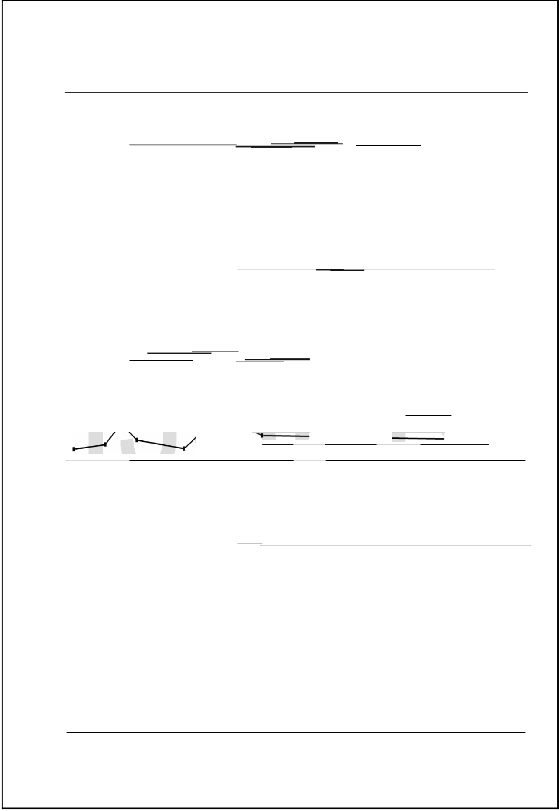
Various types of variability of AND in between the heights 6 to 7km (lower middle troposphere) are shown in Figure-1.Figure-1 shows day-to-day variability in lower middle tropospheric AND from 27 October 2009 to 6 May
2010 for morning observations. In this figure Y-axis
represents aerosol loading (Q1, calculated by equ.6) and X-
axis represents day numbers (i.e. date for each month). The
TSM data collection at Kolhapur is generally not possible
during ~mid-May to ~mid-October in any year because of
the prevailing monsoon conditions (rains and extensive cloud cover). This being a passive technique, clear sky
conditions are preferable for obtaining the vertical profiles of aerosols. Thus data coverage is for the period ~mid- October of any year to ~mid-May of the succeeding year.
For studying the seasonal variations, the year is divided into four seasons as follows:

Monsoon or rainy season:

Kolhapur city receives abundant rainfall
decreasing from early December to the mid-January (11
January 2010). This was the relatively cold period in the
winter having a lower temperature ~140C. From 11th
January Q1 values increased up to mid-February (13
February 2010). The atmosphere started warming in this
period. From mid-February Q1 values started decreasing
with lowest values of the year at mid-March (in between
10th March to 22th March). In the summer the Q1 values
started increasing from end of the March through April up to May with highest aerosol loading. Deviations from this
trend in April were observed for clear days in between cloudy days. Cumulous clouds were observed frequently in between 12th to 19th April 2010. There was no TSM data available after 6 May 2010 due to extensive cloud cover formed by the active phase of the south-west monsoon. The monthly variations were in good agreements with Hindu lunar months. (Kartika starts at ~mid-October and every succeeding Hindu lunar month starts at middle of every succeeding Gregorian month ). The monthly and seasonal variability of AND (Q1) obtained for very clear days in the present study are very well sound with the aerosol optical depth variations obtained at Mysore by Raju et al. [12].
Considering the seasonal variation of natural factors like temperature and rains Raju et al. [12], explained the experimentally observed features of aerosol characteristics as follows. The average temperature patterns

INTERNATIONAL JOURNAL OF SCIENTIFIC & ENGINEERING RESEARCH, VOLUME 4, ISSUE 1Řǰȱ ȬŘŖŗřȱȱȱ

ISSN 2229-5518

1376

for winter and summer months show significant differences. The relatively higher temperature in summer would result in enhanced aerosol generation due to primary production (bulk-to-particle conversion) and photochemical processes (secondary production) as compared to that in winter with low temperatures. During monsoon, the wet removal (scavenging) of atmospheric aerosols would be more efficient due to heavy and prolonged monsoon rains than in winter or summer seasons. The combined effect of significant wet removal of atmospheric aerosols in monsoon season, which precede the winter months, and the decreased production of small aerosols by secondary production in winter months result in an overall reduction of aerosols. In summer, there would be remarkable enhancement in the total aerosol load due to increased small particle concentration from secondary processes and large particles from primary production. In addition, the presence of substantial but infrequent rains in summer and almost total absence of rains in winter months would influence the generation, growth and loss processes of the aerosols. Further, the usual dry conditions with reduced humidity in winter months and comparatively high humidity in summer months would affect the
period. Many fluctuations were observed in the values of Q2 and Q3 from 22 December 2009 to 11 January 2010. In this period cumulus and cirrus clouds were observed frequently in between the clear sky days (cumulus clouds- middle level clouds typically found at heights between 4
Km to 6 Km; cirrus clouds- high level clouds typically found at heights greater than 6 Km). There was opposite phase relation in between the values of Q2 and Q3 for this period. In winter having lowest temperature ~140C, the values of Q2 and Q3 increased slowly up to 23th January with in phase relation between them. Again many fluctuations were observed in the values of Q2 and Q3 from
23 January 2010 to 12 February 2010. In this period also cumulus and cirrus clouds were observed frequently in between the clear days. In the face of summer season values of Q2 decreased having lowest in the month of March. After that the values of Q2 stared increasing at the face of arrival of south-west summer monsoon season. In summer season the opposite phase relation was observed in between the values of Q2 and Q3.

4.3. Comparison between morning and evening

IJSER

coagulation and growth processes of aerosols in winter and
summer months. Thus the observed seasonal variations in
the AND (in the present study) are as a result of the natural variations in the production and removal of aerosols in summer and winter. The experimental results obtained by
the present study are well agreement with theory.

4.2. The day-to-day, monthly and seasonal variability of aerosol number density per cm3 (AND) in middle and upper troposphere

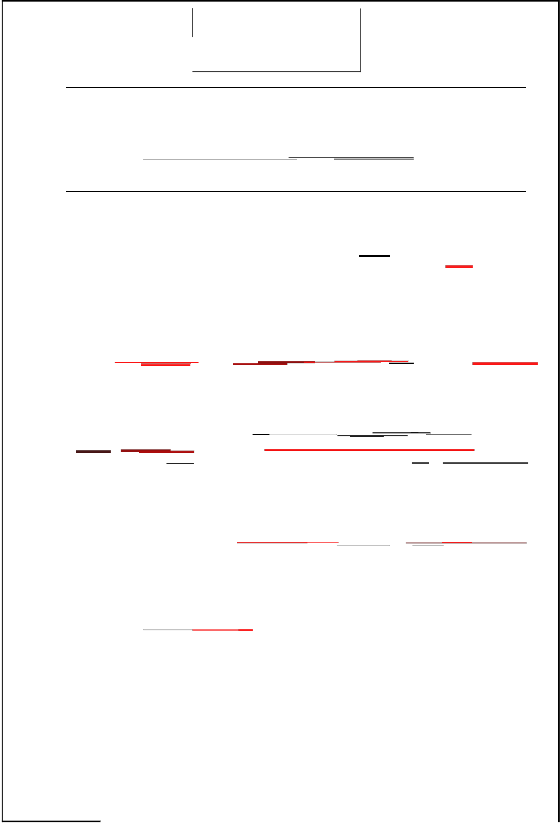
Different types of variability of AND in middle and upper troposphere are shown in Figure-2. The black and red lines show day-to-day variability in middle and upper tropospheric AND from 27 October 2009 to 6 May
2010 for morning observations respectively. The middle troposphere (heights between 8 Km to 11 Km) showed day- to-day variability from October to May with highest aerosol loading in the month of October and lowest in the middle of March. (The middle tropospheric aerosol loading is abbreviated as Q2). The upper troposphere (heights between 12 Km to 16 Km) showed day-to-day variability from October to May with highest aerosol loading in the month of October and lowest in the middle of March. (The upper tropospheric aerosol loading is abbreviated as Q3).
In the post-monsoon season the Q2 started increasing highly in the month of October with highest on 3
November 2009.The values of Q2 decreased slowly up to
24th November and then highly decreased up to 22th
December in winter. There was in phase relation in
between the values of Q2 and Q3 for all above mentioned

tropospheric aerosol number density per cm3

(AND)

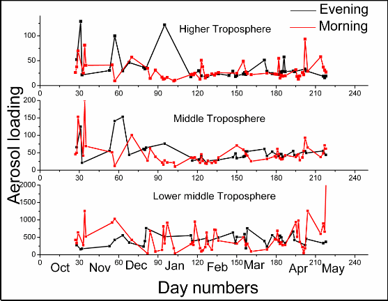
Figure-3 shows comparison between morning and evening tropospheric aerosol loading from 25 October 2009 to 10 May 2010 observations. In this figure Y-axis represents aerosol loading (Q) and X-axis represents day numbers (Day numbers 25 to 222 represent the dates from 25
October 2009 to 10 May 2010). Good agreement was observed between morning and evening aerosol loading for all the three tropospheric levels. The considerable difference in morning and evening aerosol loading was observed when there were cloudy days frequently in between clear sky days. The Lower middle tropospheric aerosol loading was ~10 times and ~15 times higher than that of middle and higher tropospheric aerosol loading respectively.

5. SUMMARY AND CONCLUSIONS

The measurements using the twilight scattering method presented in this paper suggest the following:

I. An in-phase relation has been observed between middle and upper tropospheric aerosol loading from October to January where as out of phase relation from February to May. The deviation from this trend was observed at the clear sky days in between cloudy days (i.e. when cirrus and cumulus clouds were observed frequently). More sets of observations are essential to arrive at definite conclusion.

INTERNATIONAL JOURNAL OF SCIENTIFIC & ENGINEERING RESEARCH, VOLUME 4, ISSUE 1Řǰȱ ȬŘŖŗřȱȱȱ

ISSN 2229-5518

1377

II. An in-phase relation has been observed between middle and upper tropospheric aerosol loading in post monsoon and early winter seasons, whereas out of phase relation in late winter and summer seasons. More sets of observations are essential to arrive at definite conclusion.

III. Lower middle troposphere showed well agreement

between morning and evening aerosol loading,
(exceptions of cloudy period) where as no considerable
difference observed in morning and evening aerosol
loading for middle and higher tropospheric levels.

IV. The Lower middle tropospheric aerosol loading was ~10

times and ~15 times higher than that of middle and
higher tropospheric aerosol loading respectively.

V. In the month of October lower and middle tropospheric

aerosol loading showed higher values (~50%) for 2010
than 2009 and there was about double increase in the
values of „Q‟ for the year 2010 than 2011 in the month of
January and February.

VI. The monthly variations were in good agreements with Hindu lunar months. More sets of observations are essential to arrive at definite conclusion.

[5]. Pratibha B. Mane, D. B. Jadhav, A. Venkateswara Rao, “Study of vertical distribution of stratospheric aerosol number density”, Indian Aerosol Science and Technology Association (IASTA), Vol. 20: pp. 282-286, December 2012.

[6]. Pratibha B. Mane, D. B. Jadhav, A. Venkateswara Rao, “Study of

vertical distribution of mesospheric aerosol number density”, Indian Aerosol Science and Technology Association (IASTA), Vol. 20: pp. 282-286, December 2012.

[7]. P.R. Patil, D. B. Jadhav, D. R. Jadhav, B. Padma Kumari, H. K.

Trimbake, “Automatic twilight photometer for monitoring meteor showers and vertical profiles of aerosols”, New Instruments and Technology, Advances in Remote Sensing,IUGG, TIME [ 1700 ] [ MI09/08P/B22-008 ], 2003.

[8]. Pratibha B. Mane, D. B. Jadhav, A. Venkateswara Rao,

“Semiautomatic twilight photometer design and working”, International Journal of Scientific and Engineering Research (IJSER), Vol.3, Issue-7:pp.1-7, July 2012.

[9]. Pratibha B. Mane, D. B. Jadhav, A. Venkateswara Rao, “Fast pre-

amplifier designed for semiautomatic twilight photometer”, DAV International Journal of Science (DAVIJS), Vol. 1, Issue-2: pp. 9-11, July 2012.

[10]. Bigg, E. K., “The detection of atmospheric dust and temperature

inversion twilight scattering”, Journal of Meteorology,vol.13,262-

268, 1956.

[11]. Jadhav, D. B. & A. L. Londhe, “Study of atmospheric aerosol loading using the twilight method”, J. Aerosol Sci., 23, 623-630,

1992.

IJSER

ACKNOWLEDGEMENTS: The author is grateful to the

Vice-Chancellor, Shivaji University, Kolhapur, for the
encouragement during the course of this work and also the
SERB, DST, India, for providing funds for the development of twilight photometer.

REFERENCES

[1]. D. B. Jadhav, B. Padma Kumari & A. L. Londhe, “A review on twilight photometric studies for stratospheric aerosols”, Bulletin of Indian Aerosol Science & Technology Association, 13, 1 – 17,

2000.

[2]. http://en.wikipedia.org/wiki/Kolhapur

[3]. Volz, F. E. and Goody, R. M., “The Intensity of the Twilight and

Upper Atmospheric Dust”, J. Atmos. Sci., 19,385-406, 1962.

[4]. Shah, G. M., “Study of aerosol in the atmosphere by twilight

scattering”, Tellus, 22, 82-93, 1970.

[12]. N. V. Raju, B S N Prasad, B Narasimhamurthy and M Thukarama,

“Meteorological and anthropogenic influences on the atmospheric aerosol characteristics over a tropical station Mysore (120N)”, Indian J. Radio & Space Phys., Vol. 29, pp. 115-126, June

2000.

Corresponding author:
Space Research Centre, Department of Physics, Shivaji University, Kolhapur-416 004, Maharashtra state, India. Email: pratibhabm263@gmail.com

INTERNATIONAL JOURNAL OF SCIENTIFIC & ENGINEERING RESEARCH, VOLUME 4, ISSUE 12, DECEMBER-2013

ISSN 2229-5518

1378

October

2009

11 ._/

	I	I	I	I	I	I	I	I	I	I	I	I	I
0	4	6	10	12	14	16	18	20	22	24	26	28	30

November

:=. 2009

December

209

c I I

I I I I I I I I

·- 0

4 6 10 12 14 16 18 20 22 24 26 28 30

ro 11

I I I I I I I

0 4 6 10 12 14 16 18 20 22 24 26 28 30

tJ)

I I I I I I I I I

2010

I I

Q) 0 10 12 14 16 18 20 22 24 26

1 1

28 30

March

: I I I I I :

0 4 6 8 10 12 14 16 18 20 22 24 26 28 30

April

1 1 2010

I I I I

0 4 6 10 12 14 16 18 20 22 24 26 28 30

May

Day numbers

Figure-1: Varies types of variability of AND in between the heights 6 to 7km

2010

INTERNATIONAL JOURNAL OF SCIENTIFIC & ENGINEERING RESEARCH, VOLUME 4, ISSUE 12, DECEMBER-2013

ISSN 2229-5518

-+--Middle troposphere (Q) October

11 -+-- Upper troposhere (Q ) 2009)/

1379

	I	I	I	I	I	I	I	I	I	I	I	I	I
0	4	6	10	12	14	16	18	20	22	24	26	28	30

November

I 2009

	I	I	I	I	I	I	I	I			I	I
0	4	6	10	12	14	16	18	20	22	24	26	28	30

December

11 2009

I I I I I

0 4 6 10 12 14 16 18 20 22 24 26 28 30

ro 0 2

l"'-: I

I : : :

January

2010

February

11 =: :

I ::::= I I I I I I

; 2010

I I I

(/) 0

2 4 6 10 12 14 16 18 20 22 24 26 28 30

0 March

I I I I I I I

0 4 6 8 10 12 14 16 18 20 22 24 26 28 30

April

:::; : :;:: I I I : I I I I

0 2 4 6 10 12 14 16 18 20 22 24 26 28 30

May

I 2010

I I I I I I I I I I I I I

0 4 6 10 12 14 16 18 20 22 24 26 28 30

Day Numbers

Figure-2: Varies types of variability of AND in middle and upper troposphere

IJSER ©201 3

htt:IIWWW .ISer.org

INTERNATIONAL JOURNAL OF SCIENTIFIC & ENGINEERING RESEARCH, VOLUME 4, ISSUE 1Řǰȱ ȬŘŖŗřȱȱȱ

ISSN 2229-5518

1380

IJSER

Figure-3: comparison between morning and evening tropospheric aerosol loading