Straight Line Detection AndReal -Time Line detection Using OpenGL

International Journal of Scientific & Engineering Research, Volume 5, Issue 3, March-2014 1023

ISSN 2229-5518

1Moumita Ghosh,

University Institute Of Technology,

(The University Of Burdwan) Pin -712104,India mou2005be@gmail.com

2Himadri NathMoulick,

CSE, Aryabhatta Institute of Engg& Management, Durgapur, PIN-713148, India

himadri80@gmail.com

ABSTRACT-Line recognition is an important aspect in image processing. Many line detection algorithms were introduced. Hough Transform for line detection is difficult to accelerate using the GPU because it essentially requires rasterization of sinusoids into a high- resolution raster of accumulators, which is not a suitable task for GPU. In this paper, a GPU implementation of the PClines - a new parameterization of lines for the Hough Transform. PClines are a point-to-line-mapping . The detection of lines uses the graphics processor to rasterize lines into a rectangular frame buffer which is a task very natural and effective on the GPU. The OpenGL 3.3 pipeline is used to efficiently perform the whole of the PClines-based Hough Transform on the GPU. Experimental evaluation shows that even for high-resolution input images with complicated content, the line detector performs easily in real time.

Keywords- Line detection, width estimation, edge, Helmholtz principle ,Acontrario detection,

detection.

I.INTRODUCTION
Image processing is one of the most important areas in computer science and engineering. One of the main goals of image processing is to be able to identifyobjects of the image. Objects in a computer image are identified by their edges. These edges could be straight lines or curved lines. Many algorithms were used todetect a line in gray-scaled images as well as coloredimages. Each algorithm has some conditionsandconstraints to deal with. Guido introduces an algorithmto detect a line based on a weighted minimum mean square error formulations [1]. This algorithm works with matrices and uses a set of matrix operations such astranspose and multiplications.
The Hough transform is a well-known tool for detecting shapes and objects in raster images. Originally, Hough [6] defined the transformation for detecting lines; later it was extended for more complex shapes, such as circles, ellipses, etc., and even generalized for arbitrary patterns [1].
When used for detecting lines in 2D raster images, the Hough transform is defined by a parameterization of lines: each line is described by two parameters.[3] The input image is preprocessed and for each pixel which is likely to belong to a line, voting accumulators corresponding to lines which could be coincident with the pixel are increased. Next, the accumulators in the
parameter space are searched for local maxima above a given threshold, which correspond to likely lines in the original image.[3] The Hough transform was formalized by Princen et al. [14] and described as an hypothesis testing process.
Another approach based on repartitioning the Hough space is represented by the Fast Hough Transform (FHT) [8]. The algorithm assumes that each edge point in the input image defines a hyperplane in the parameter space. These hyperplanes recursively divide the space into hypercubes and perform the Hough transform only on the hypercubes with votes exceeding a selected threshold. This approach reduces both the computational load and the storage requirements.[7] Using principal axis analysis for line detection was discussed by Rau and Chen [15]. Using this method for line detection, the parameters are first trans- ferred to a one-dimensional angle-count histogram. After transformation, the dominant distribution of image features is analyzed, with searching priority in peak detection set according to the principal axis.[11] There exist many other ac- celerated algorithms, more or less based on the above mentioned approaches; e.g. HT based on eliminating of particle swarm [2] or some specialized tasks like iterative RHT [9](Randomized Hough Trans-form) for incomplete ellipses and N-Point Hough transform for line detection [10].
Segments in images give important information about their geometric content. Segments as features can help in several problems.[33] To cite just a few: stereo analysis [26], classification tasks like on-board selection of relevant im- ages

International Journal of Scientific & Engineering Research, Volume 5, Issue 3, March-2014 1024

ISSN 2229-5518

[35], crack detection in materials [36], stream and roadbeds detection [50], and image compression [18].
They serve as a basic tool to find sailing ships and their V-shaped wakes [8, 29], to detect filamentous structures in cryo-electron microscopy images [52], or to detect lines in forms [51]. On other problems line segments are just a con- venient way to handle structure, e.g., in [19, 30, 48] line networks are approximated by small segments.Segments are one of the basic shapes in graphics. The gestalt school [28] has gone so far as to analyze human per- ception with line drawings essentially made of straight seg- ments. Most human-made environments and in particular ar- chitectures are based on alignments. [40]All photographs made in those environments show alignments as an essential per- spectivefeature.It would seem that such a basic problem as segment de- tection is a simple one and has been tackled once for ever. [40]We hope to convince the reader that it has not. We intend to show that it is a more complex event than anticipated in the former theories. [46]This explains why, to the best of our knowledge, all existing algorithms have serious drawbacks. Worse than that, they do not deliver a result reliable enoughto found a hierarchical image analysis. [33]Three issues have tobe solved: over-detection (false positives), under-detection (false negatives) and the accuracy of each detection.Line detection is an integral part of many image processing tasks such as camera calibration, object detection or marker localization (bar codes, QR codes, augmented reality mark- ers), and many more. Because some of these tasks are per- formed online, fast line detection is not only desirable but sometimes necessary. [42]This paper is about real-time detec-tion of lines based on a parameterization using parallel coor- dinates (PC) and implemented on GPU using OpenGL shad- ing language. Other GPU implementations of the Hough Transform exist, however the PClinesparametrization is per- fectly suitable for OpenGL implementation because it re- quires only line rasterization. The goal of the presented re- search is to maximally utilize contemporary graphics chips for the task of detecting straight lines in raster images.[29]
II. LINE RECOGNITION THEORY AND ALGORITHMS

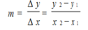
The equation of a line is y=mx+b, where m is the slope of a line, and b is the y-intercept. The slope
(1)
for any two points (x1 ,y1 ), (x2 ,y2 ) that lie on the line. On the computer graphic devices such as screen, printer and plotter or
any image file like BMP and JPEG, an image consists of pixels. The line that is drawn using grids is actually an approximation of the ideal/actual line.[39]This line is formed by a set of adjacent straight lines that are close to each other using corner pixels.
In this paper, an algorithm to find the properties of a line using the properties of those actual straight line segments that form a line is presented.[27]
The slope of an ideal line is as in (1). In the first octant where the slope is between 0 and 1, i.e.,
0 ≤ m ≤ 1 (2)
Substituting for m in (2) yields
0 ≤ Δ y ≤ Δ x (3)
In the grid layout, all computations are done using integers. [11] Even if you are using floating point
calculations, once you need to know if the grid point is illuminated or not, rounding the value to an integer number is usually performed. So the ideal line isrepresented on the grid layout using a set of straight line
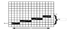
segments. If the first and fourth octants of the plane are considered, these straight line segments are horizontal
lines. If the line lies in the second or third octant, thesestraight lines are vertical lines. In this paper, our approach deals with the first octant, so we are considering horizontal lines. By this, the ideal line is formed using a number of straight lines. The graph of a line on the grid layout looks like stairs, as shown in Figure 1

Fig.1. Horizontal line segments

International Journal of Scientific & Engineering Research, Volume 5, Issue 3, March-2014 1025

ISSN 2229-5518

Fig.2. Ideal line drawn on a grid layout

Each increment in the y-direction is only one pixel, while the increment in the horizontal direction varies according to the end points of the line.[22] The number of horizontal lines segments is Δy. The length of each horizontal line segment depends on Δy and Δx.The line that is drawn on a grid layout is formed by adjacent equal segments {S1 , S2 , …, S n } if each line segment has the same slope as the ideal line. Figure1shows an ideal line with a number of horizontal line segments representing the approximation of this line. This means that the slope for each segment is equal to the slope of the whole line. The slope of each segment is
(4)
Since integer computations are performed, the slope isactually an approximation. The vertical increment is

always 1.Δy = 1 as it is a grid layout, Therefore
(5)
The ideal line passes at the middle of each vertical linesegment.[43]This line passes closely to the middle of every vertical line segment (Δy =1), which is
(6)
The slope of the segment that passes at the middle of thevertical increment is
(9)

A.Straight line detection algorithm

The algorithm is used to recognize a straight line in a graphic image.[37] It works for the first octant of the plane,
where the slope is between 0 and 1. Generalizing thealgorithm for the whole plane is straight forward. The
main advantage of the algorithm is its simplicity and robustness. [34]The algorithm can detect any line that is
continuous in the plane.The data structures required for the algorithm are a matrix for the image, a bit matrix for visited pixels, the number of rows and columns of the matrices which aredependent on the size of the image.A new data type is used to save the values of the line. It has four integer values for the starting and ending points. [22]To save computational time, the length of linesegment is saved as a member of this new data type. Inorder to keep track of all lines within the same image, a list of lines data structure is required.[24]
The algorithm is shown in Algorithm 1. The algorithm loopsthrough all pixels of the image in a row-major order. It
checks if the pixel is part of a line and is not visitedthen it starts a sequence of operations to find the line.[45]
These operations start by finding the first horizontal line segment and consider it as a temporary line. [39]Then from the end of that segment in the next row, it checks for another horizontal line. If another horizontal line isfound, the length of the new horizontal line is checked.Its length should be between the length of the first horizontal segment and its double length. [29]If theconditions fail, that means there is no more horizontal
Line_Recognition_Algorithm1 (Input: Matrix, Output: Lines-List)
This leads to

(7)
// Matrix: matrix representation of the image.
// Lines-List: a list of recognized lines from the image
begin

(8)
The middle horizontalsegments lengths have values close to the double of the first and last horizontal segments lengths i.e[45]
for i=1 to image-height for j = 1 to image-width
if ((Matrix[i][j] ==lineColor) && Not done[i][j] )

International Journal of Scientific & Engineering Research, Volume 5, Issue 3, March-2014 1026

ISSN 2229-5518

set MoreSeg to TRUE;
r = i c= j
find a horizontal segment at (r, c)
save the horizontal segment parameters into Temp-Line
set the length of the horizontal segment to len set maxlen to double the length of segment
change the status of those pixels to visited while there are
MoreSeg
if direction is RIGHTDOWN
// direction of the first octant
find next horizontal segment at (r+1, Previous segment c+1)
end if
if ( length of the segment is between len and maxlen)
Change the end point of the Temp-Line to be the endpoint of the new segment Change the status of those pixels to visited else
MoreSeg = FALSE
end if
end while
add temporary line to the Lines-List endif
end
All algorithms that are used for line recognition and detection in image processing involve very expensive
operations like floating-point calculation and matrixoperations.[22] It is known that these operations are very time consuming and using them will definitely slow down these algorithms significantly.[19] On the other hand,our algorithm uses only simple integer arithmetic. In addition to that, our algorithm involves the simplest forms of arithmetic operations namely, additions,comparisons and logical operations. [41]There are no multiplications or divisions. Therefore, our algorithm has a great value in line recognition and image
processing due to its simplicity and efficiency.

B. Straight line detection using Principal component analysis

(PCA)

PCA is a well-known metric method .

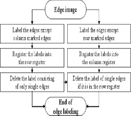
Fig. 3.

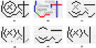
Fig.4. Example of edge labeling: (a) edge image, (b) blue, red, green, and black is column, row, single, and cross primitive

International Journal of Scientific & Engineering Research, Volume 5, Issue 3, March-2014 1027

ISSN 2229-5518

respectively, (c) is the edge image except column marked edges, (d) is the edge image except row marked edges. After eliminating gray points in (c) and (d), the edges consisting of only single primitives remain in column edge image, (f) while row edge image and (e) does not have such edges. (For interpretation of references in color in this figure legend, the reader is referred to the web version of this article.)
PCA is a well-known metric method that produces the base axes of a distribution of data (Duda et al., 2001).
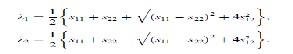
Given an ideal straight line in two dimension, it has some principal components deduced from the eigenvectors and eigenvalues of the scatter matrix. The eigenvector means one main direction of the distribution of the pixels of a line and the eigenvalue means how long the distribution is. Generally, the first eigenvalue is larger than the second one, so that, in the case of ideal straight line, the second eigenvalue should be zero.[35] However, a digital line is repre- sented stepwise, so that the second eigenvalue of the line cannot be zero. [32]The tolerance for that case will be addressed and determined in the next section. The scatter matrix is as follows:

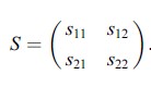
If n is the number of pixels in a line and (xi,yi ) is the coor- dinates of the ith pixel of the line,
The large eigenvalue k1 and the small eigenvalue k2 of the scatter matrix are

We can only know the proportion of the elements of theeigenvector, and so the angle of the line, h is defined as

If an image has k edge pixels, row and column edge sep- aration has O(2k) = O(k) because every pixel is compared to the next and below pixel. After that, if the edge imageshave l lines and the average length (pixels) of lines is a,thelabeling processing takes O(la2), because in the worst case, every pixel of a line has its own label so that it will be compared to one another.[45]However, PCA is an arithme-tic calculation and it has O(1). [44]Therefore, the sum of the order is O(k) + O(la2) · O(1) = O(k) + O(la2), but roughlyk = la; so the time complexity is O(ka).

C. PClines: Line Detection using ParallelCoordinates

Parallel coordinates (PC) were invented in 1885 by Maurice d’Ocagne [d’Ocagne 1885] and further studied and popular- ized by Alfred Inselberg [2009]. The coordinate system used for

International Journal of Scientific & Engineering Research, Volume 5, Issue 3, March-2014 1028

ISSN 2229-5518

representing geometric primitives in parallel coordinates is defined by mutually parallel axes.[33] Each N -dimensional vector is represented by (N − 1) lines connecting the axes - see Fig. 6. In this text, we will be using an Euclidean plane with a u- v Cartesian coordinate system to define positions of points in the space of parallel coordinates.[12] For defining these points, a
notation (u, v, w) P 2 will be used for homogeneous coordinates in
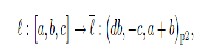
(denoted as [a, b, c]) and its representing point ℓ can be defined
by mapping:
the projective space P2 and (u, v)E 2 will be used for Cartesian coordinates in the Euclidean space E2 .In the two-dimensional case, points in the x-y space are rep- resented as lines in the space
where d is the distance between parallel axes x′
and y′.
of parallel coordinates. [24] Representations of collinear points intersect at one point - the representation of a line (see Fig. 5). Based on this relation- ship, it is possible to define a point-to-line mapping between

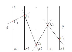
Fig.5. Representation of a 5-dimensional vector in paral- lel coordinates. The vector is represented by its coordinatesC1 , . . . , C5 on axes x′1 , . . . , x′5, connected by a complete poly-line (composed of 4 infinite lines).

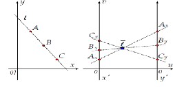
Fig.6.Three collinear points in parallel coordinates: (left) Cartesian space and (right) space of parallel coordi- nates. Line ℓ is represented by point ℓ in parallel coordi- nates[39]
the original x-y space and the space of parallel coordinates.[11] For some cases, such as line ℓ : y = x, the corresponding point ℓ lies in infinity (it is an ideal point). Projective space P2 (contrary to the Euclidean E2 space) provides coordi- nates for these special cases. [33]A relationship between line ℓ :ax + by + c = 0

1 .Parameterization “PClines” for Line Detection

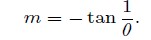
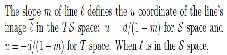
This section gives a brief overview of the “PClines” param- eterization introduced in [Dubská et al. 2011]. In the fol-lowing text, we will use the intuitive slope-intercept line equation y
= mx + b. Using thisparameterization, the`orrespondi´g point ℓ
in the parallel space has coordinates d, b, 1 − m P2 . The line’s representation ℓ is between theaxes x′ and y′ if and only if
−∞< m < 0. For m = 1, ℓ is an ideal point (a point in infinity). For m = 0, ℓ lies on the y′ axis, for vertical lines (m = ±∞), ℓ lies on the x′ axis.
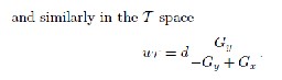
Besides this space defined by parallel axes x′ , y′ (further referred to as straight, S ), we propose using a twisted (T ) system x′ , −y′ , which is identical to the straight space, ex- cept that the y′ axis is inverted. In the twisted space, ℓis between the axes x′ and −y′ if and only if 0 < m <∞. By combining the straight and twisted spaces, the whole T S plane can be constructed. The original x-y image with three points A, B, and C and three lines ℓ1 ,ℓ2 , and ℓ3 coincident with the points. [29]The origin of x-y is placed into the middle of the image corresponding T S space. It should be noted that a finite part of the u-v plan is sufficient:

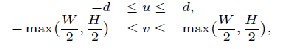
where W and H are the width and height of the input rasterimage, respectively.[19]
Any line ℓ : y = mx + b is now represented either by point ℓS in the straight half or by ℓT in the twisted part of the u-v plan :

International Journal of Scientific & Engineering Research, Volume 5, Issue 3, March-2014 1029

ISSN 2229-5518

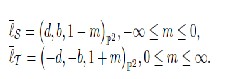
Consequently, any line ℓ has exactly one image ℓ in the T Sspace; except for cases that m = 0 and m = ±∞, when ℓlies in both spaces either on axis y′ or x′ . That allows the T and S spaces to be “attached” to one another. [30] The spaces attached along the x′ axis. Attaching also the y′ and −y′ axes results in an enclosed Möbiusstrip.This parameterization can be used for detecting lines using the standard Hough transform procedure, as depicted in Algorithm 2. The space S(u, v) is discretized directly according
Algorithm 2 .Detection of lines using parallel coordinates. Input : Input image I with dimensions W, H
Output :Det,ected lines L={(m1,b1),…..}
1: S(u, v) ← 0, ∀u ∈ {−d, . . . , d}, v ∈ {vmin , . . . , vmax }
2: for all x ∈ {1, . . . , W }, y ∈ {1, . . . , H } do
3: if I (x, y) is an edge then
4: rasterize line in the S space
5: rasterize line in the T space
6: end if
7: end for
8: L ←{}
9: L = (m(u), b(u, v))|u ∈ {−d, . . . d}∧
v∈ {vmin , . . . , vmax } ∧ S(u, v) is a high local max.}
to Eq. (2); other discretizations - denser or sparser – wouldbe
possible by just linearly mapping the u and v coordinatesused in the algorithm.[20] The condition used in codeline 3is application-specific and it typically involves an edge de-tection operator and thresholding. [39] The lines rasterized incodeline 4 and 5, in fact, constitute a two-segment polylinedefined by three points: (−d, −y) − (0, x) − (d, y). Codeline 9 scans the space of accumulators S for local maxima above agiven threshold - this is a standard Hough transform step.[30]
III. REAL –TIME LINE DETECTION USING Open GL
In the presented GLSL implementation, the following shaderprograms are used:Imagepreprocessing program in case the input image re-quires preprocessing, namely conversion to greyscale.This program is optional.Accumulation program for accumulating the edges’ votesfrom the input image to the T S space.Detection program for detecting local maxima in the T Sspace.Both the image preprocessing and the T S space accumula- tion programs are implemented via rendering to a texture. The (optional) preprocessing step is done by simple screenquadrenderingMost of the T S space accumulation is done by a geometry shader. A point for every pixel of the input image is rendered by geometry instancing. Builtin variables glVertexID and glInstanceID specify the point coordinates.[34] The geometry shader reads the input image at the specified coordinatesand thresholds the value to determine whether it is an edge. [44]The output of the geometry shader is a three-point line strip that is rasterized to the T S space. The u coordinates of the points are
fixed {−1, 0, 1} and the v coordinates are based on the input
point coordinates (x, y) (see Section 2.1). The T S space is accumulated using additive blending into a floating-point texture.The maxima detection is also performed by a geometry shader. [39] A point is rendered for each pixel of the T S space (stored in the texture) and the geometry shader checks the small neighbourhood of this pixel to see whether it is a lo- cal maximum. In that case, the detected line is returned by the transform feedback. The maxima detection could be implementedseparably using two passes and one temporary texture. [40] However, experiments have shown that the single pass detection performed faster for all used neighbourhood sizes.

A.Harnessing the Edge Orientation

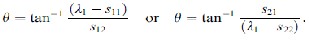
O’Gorman and Clowes [1976] improve the basic θ-̺param- eterization with their idea of not accumulating values for all discretized values of θ but for a single value of θ, instead. The appropriate θ for a point can be obtained from the gra- dient of the detected edge present at this point [Shapiro and Stockman
2001].One common way to calculate the local gradient direction of the image intensity is by using the Sobel operator. [38]Sobelker- nels for convolution are as follows: Sx = [1, 2, 1]T
· [1, 0, −1] and Sy = [1, 0, −1]T · [1, 2, 1]. Using these
convolution ker- nels, two gradient values GxandGy can be obtained for any discrete location in the input image. Based on these, the gradient’s direction is θ = arctan(Gy /Gx ). The line’s incli-
nation in the slope-intercept parameterization m-b is related

International Journal of Scientific & Engineering Research, Volume 5, Issue 3, March-2014 1030

ISSN 2229-5518

Algorithm 3 Geometry Shader Using Edge Orientation

Input: Image I with dimensions W, H , radius r and d=1 Output: Accumulator space S (refer to Alg. 1)
1: for all x ∈ {1, . . . , W }, y ∈ {1, . . . , H } do

2: Gx = (I ∗Sx )(x, y)
3: Gy = (I ∗Sy )(x, y)
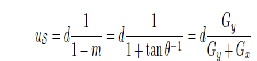
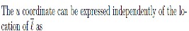
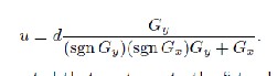
4: u = Gy/ sgn(Gx ) sgn(Gy )Gy + Gx
5: if Gx +Gy>τ then

6: uL = u + r, uR = u − r
7: if uL<= 0 ∧uR<= 0 then
8: emit vertex (uL , (y + x) ∗uL + x, 0)
9: emit vertex (uR , (y + x) ∗uR + x, 0)
10: else if uL>= 0 ∧uR>= 0 then
11: emit vertex (uL , (y − x) ∗uL + x, 0)

12: emit vertex (uR , (y − x) ∗uR + x, 0)
13: else if uL<−1 ∨uR> 1 then
It should be noted that contrary to the “standard” θ-̺ pa- rameterization, no goniometric operation is needed to com- pute the horizontal position of the ideal gradient in the accu- mulator space.[45] In order to avoid errors caused by noise and the discrete nature of the input image, accumulators within a suitable interval 〈u − r, u + r〉 around the calculated angle (or more
precisely u position) are also incremented. [9]That - unfortunately
-introduces a new parameter of the method - radius r. However, experiments show that neither the ro- bustness nor the speed is affected notably by the selection of r.The algorithm of line detection taking into account the edgeorientation is depicted by Algorithm. 3. Although the T S space is a plane, three dimensional space is involved. The third coordinate is used in one special case illustrated by Figure 4. It is the situation which occurs if the rendered part of the polyline around the estimated u is outside of interval [−d, d]. Such a situation results in the
necessity of rendering two separate lines. Instead of calculating all four endpoints of the lines, only three vertices are emitted with different z- coordinates and the back clipping plane of the OpenGL view frustum is used to clip the polyline.[49]
14: if uL<−1 then
15: uL =uL + 2
16: end if
17: if uR> 1 then
18: uR =uR− 2
19: end if
20: z = (1 − r)/r
21: emit vertex (−1, −y, (z(1 + uR ) − 1)/uR )
22: emit vertex (0, x, z)
23: emit vertex (1, y, (1 −z(1 −uL ))/uL )
24: else
25: emit vertex (uL , (y + x) ∗uL + x, 0)
26: emit vertex (0, x, 0)

International Journal of Scientific & Engineering Research, Volume 5, Issue 3, March-2014 1031

ISSN 2229-5518

27: emit vertex (uR , (y − x) ∗uR + x, 0)
28: end if
29: end if
30: end for
IV.EXPERIMENTAL RESULT
This section presents the experimental evaluation of the pro-posed algorithm. Though the aim of this paper is mainly the GPU speed- up, it is important to mention the accuracy ofPClinesdetection - referred to in Section ASection B contains the results achieved
vertices A−y and Ay are calculated according to the required
lengths of the line segments.

A.Accuracy Evaluation

The line localization error was measured on automatically generated data and calculated as the Euclidean distance from the ground truth. For comparison, Hough trans- form using θ-ρ and m-b (slope-intercept) parametrizationswas used. Figure 9 shows the dependency of the detec-tion error on the line’s slope for all the three parameter- izations. The test was performed on images 512 × 512 pixels and lines generated with random θ in 5◦ intervals. The measurements show that the θ-̺ parameterization dis-
cretizes the space evenly; PClines are about as accurate as θ-̺
by the GLSL implementation of PClines presented in this
paper.[10]The following hardware was used for testing (in bold
for θ∈ {45◦
, 135◦
, 225◦
, 315◦
} and more accurate atθ∈
face is the identifier used in the text):
GTX 480 - NVIDIA GTX 480 in a computer with IntelCore i7-
920, 6GB 3×DDR3-1066(533MHz) RAM;
GTX 280 - NVIDIA GTX 280 in a computer with IntelCore i7-
920, 6GB 3×DDR3-1066(533MHz) RAM;
GT 130M - NVIDIA GT 130M mobile GPU in a lap-top computer with Intel Core 2 DUO T6500, 2× 2GBDDR2
399MHz RAM;HD 5970-1 - AMD Radeon HD5970 (single core used) ina computer with Intel Core i5-660, 4GB 3×DDR3-
1066(533MHz) RAM;HD 5970-2 - AMD Radeon HD5970 (both cores used) in a computer with Intel Core i5-660, 4GB
3×DDR3-1066(533MHz) RAM; andi7-920 - Intel Core i7-920,
6GB 3×DDR3-1066(533MHz)RAM - the same computer is used for testing theGTX 480 and GTX 280

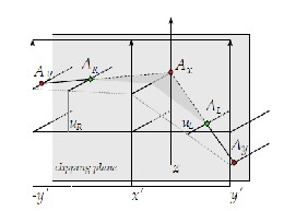
Fig.7. Three vertices used for rendering two separateline segments. The middle point Ax has its z-coordinate calculated as (1−r)/r, where r is the radius rendered around the
predicted u (this restricts r to be smaller than d). The depths of
{0◦ , 90◦ , 180◦ , 270◦ }; the m-b parameterization is the least
accurate of the three evaluated methods. One should refer to
[Dubská et al. 2011] for more details.[10]

B.Performance Evaluation on Real-Life Images

As the dataset for this test real photographs with different amounts of edge points and different dimensions were used. [11]The images are sorted according to the number of edge points detected by the Sobel filter.[12]
The presented algorithm (further referred to as PClines) was compared to a software implementation of the “stan- dard” θ-̺ based Hough transform taken from the OpenCVlibrary1 and parallelized by OpenMP and slightly optimized.[15]The results are reported in Figure 10. The measurements ver- ify that the computational complexity depends mostly on the number of edge points extracted from the input image and the edge-detection phase is linearly proportional to the im- age resolution, which causes nonlinearity in the graph. [16]The GPU-accelerated implementations are notably faster than the software implementation. [7] A detailed comparison of the GPU- accelerated implementations is shown in Figure 12.

International Journal of Scientific & Engineering Research, Volume 5, Issue 3, March-2014 1032

ISSN 2229-5518

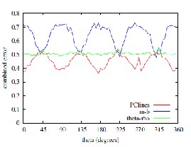
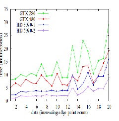
Fig.8. Line localization error as it depends on the lines’slope. For x on the horizontal scale, the lines’ slope in de- grees is at interval 〈x, x + 5). Red: PClines; Green: θ-̺; Blue: m-b. Average error of the 5 least accurate lines, (i.e. a pessimistic error estimation).

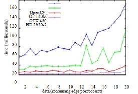
Fig.9. Performance evaluation of computational complex-ity tested on real-world images. The GLSL implementation is compared to a parallelized OpenCV implementation (us- ing all cores of the i7-920). Figure 10 shows the individual images (horizontal axis of this graph).

Fig. 10. Images used in the test. The number in the top-left corner of each thumbnail image is the image ID - used on thehorizontal axis . The bottom-left corner of each thumbnail image states the number of edge points and pixelresolution of the tested image.
Fig.11. Performance evaluation of the GLSL implementa-tion using different high-end graphics hardware.
IV.CONCLUSION
All algorithms that are used for line recognition and detection in image processing involve very expensive operations like floating-point calculation and matrixoperations. It is known that these operations are very time consuming and using them will definitely slow down these algorithms significantly.[20] On the other hand,our algorithm uses only simple integer arithmetic. In addition to that, our algorithm involves the simplest forms of arithmetic operations namely, additions,comparisons and logical operations. There are no multiplications or divisions. [19]Therefore, our algorithm has a great value in line recognition and imageprocessing due to its simplicity and efficiency.This paper presents an OpenGL 3.3 implementation of
the PClines line detector. Contrary to the “standard” θ-̺ pa-
rameterization which requires rasterization of sinusoids into the Hough accumulator space, PClinesare a point-to-line- mapping. That allows for a very efficient use of the GPU for accumulation of the votes in the Hough space.The results show that PClines can be used for real-time de- tection of lines, even in complex images of high resolutions. [3] The accuracy of the parameterization notably outperforms the original Hough’s slope-intercept parameterization and it is equal or more accurate than the commonly used θ-̺ pa- rameterization. Together with its ability
to directly detect sets of parallel or mutually coincident lines, PClines seem very attractive for use in various applications.[2] One advan-tage of the presented solution is its ability to avoid using of CUDA or OpenCL which are still facing compatibility
issues.[37]The simplicity of the algorithm is not only suitable for

International Journal of Scientific & Engineering Research, Volume 5, Issue 3, March-2014 1033

ISSN 2229-5518

imple- mentation in OpenGL which is presented here. In the near future, we are considering experiments on programmable hardware (FPGA). Another interesting topic of future study can be porting the algorithm presented here to older versions of the OpenGL pipeline. Such ports can be welcome in con- temporary smartphones and other mobile and ultramobile devices supporting OpenGL ES.
REFERENCES

[1] M.A. Fischler, “The Perception of Linear Structure: AGeneric Linker,” Image Understanding Workshop, pp.1,565-1,579. San Francisco: Morgan Kaufmann Publishers,1994.

[2] D. Geman and B. Jedynak, “An Active Testing Model forTracking Roads in

Satellite Images,” IEEE Trans. Pattern

Analysis and Machine Intelligence, vol. 18, no. 1, pp. 1-14,Jan. 1996.

[3] Mark J. Carlotto, “Enhancement of Low-ContrastCurvilinear Features in

Imagery”, IEEE Transactions OnImage Processing, Vol. 16, No. 1, pp. 221-228,

January2007.

[4] J.B. Subirana-Vilanova and K.K. Sung, “Multi-ScaleVector-Ridge- Detection for Perceptual OrganizationWithout Edges,” A.I. Memo 1318, MIT

ArtificialIntelligence Lab., Cambridge, Mass., Dec. 1992.

[5] T.M. Koller, G. Gerig, G. Székely, and D. Dettwiler,“Multiscale Detection of

Curvilinear Structures in 2-D and

3-D Image Data,” Fifth Int’l Conf. Computer Vision, pp.864-869. Los Alamitos, Calif: IEEE CS Press, 1995.

[6] L.A. Iverson and S.W. Zucker, “Logical/Linear Operatorsfor Image Curves,”

IEEE Trans. Pattern Analysis and

Machine Intelligence, vol. 17, no. 10, pp. 982-996, Oct.1995.

[7] J.B.A. Maintz, P.A. van den Elsen, and M.A. Viergever,“Evaluation of Ridge

Seeking Operators for Multimodality

Medical Image Matching,” IEEE Trans. Pattern Analysisand Machine

Intelligence, vol. 18, no. 4, pp. 353-365, Apr.1996.

[8] C. Steger, “An unbiased detector of curvilinear structures,”IEEE Trans. Pattern Anal. Machine Intell., vol. 20, pp. 113-

-125, Feb. 1998.

[9] J. H. Van Deemter, J. M. H. Du Buf, “SimultaneousDetection Of Lines And

Edges Using Compound GaborFilters”, International Journal of Pattern

Recognition andArtificial Intelligence, Vol. 14, No. 6, pp. 757-777, 2000.

[10] Z.-Q. Liu, J. Cai, and R. Buse, Handwriting Recognition:Soft Computing and

Probabilistic Approaches, pp. 31-57, Springer, Berlin, 2003.

[11]. Deriche, R., Faugeras, O.: Tracking line segments. J. Image Vis.Comput.

8(4), 261–270 (1990)

[12]. Desolneux, A., Moisan, L., Morel, J.-M.: Maximal meaningfulevents and applications to image analysis. Technical Report 2000-22, CMLA, ENS-

CACHAN (2000). Availableat http://www.cmla.ens- cachan.fr/fileadmin/Documentation/Prepublications/2000/CMLA2000-22.ps.gz [13]. Desolneux, A., Moisan, L., Morel, J.-M.: Meaningful alignments.Int. J. Comput. Vis. 40(1), 7–23 (2000)

[14]. Desolneux, A., Moisan, L., Morel, J.-M.: Edge detection byHelmholtz principle. J. Math. Imaging Vis. 14(3), 271–284 (2001)

[15]. Desolneux, A., Moisan, L., Morel, J.-M.: From Gestalt Theory toImage Analysis. Interdisciplinary Applied Mathematics, vol. 35.Springer, New York (2007)

[16]. Faugeras, O., Deriche, R., Mathieu, H., Ayache, N.J., Randall, G.:The depth and motion analysis machine. PRAI 6, 353–385 (1992)

[17]. Fernández, F.:Mejoras al detector de alineamientos. Technical Report,InCO,

Universidad de la República, Uruguay (2006)

[18]. Fränti, P., Ageenko, E.I., Kälviäinen, H., Kukkonen, S.: Compressionof line drawing images using hough transform for exploitingglobal dependencies. In:

JCIS 1998 (1998)

[19]. Geman, D., Jedynak, B.: An active testing model for trackingroads in satellite images. IEEE Trans. Pattern Anal. Mach. Intell.

18(1), 1–14 (1996)

[20]. GiaiCheca, B., Bouthemy, P., Vieville, T.: Segment-based detectionof moving objects in a sequence of images. In: ICPR94,

pp. 379–383 (1994)

[21]. Grompone von Gioi, R., Jakubowicz, J.: On computationalgestalt detection thresholds. J. Physiol.—Paris (2008, to appear).

http://www.cmla.ens- cachan.fr/fileadmin/Documentation/Prepublications/2007/CMLA2007-26.pdf

[22]. Hough, P.V.C.: Method and means for recognizing complex patterns.U.S.

Patent 3,069,654, 18 December 1962

[23.]Igual, L.: Image segmentation and compression using the tree ofshapes of an image. Motion estimation. Ph.D. Thesis, UniversitatPompeuFabra (2006)

[24]. Igual, L., Preciozzi, J., Garrido, L., Almansa, A., Caselles, V.,Rougé, B.: Automatic low baseline stereo in urban areas. Inverse

Probl. Imaging 1(2), 319–348 (2007)

[25]. Illingworth, J., Kittler, J.: A survey of the Hough transform. Comput.Vis. Graph. Image Process.44(1), 87–116 (1988)

[26]. Ji, C.X., Zhang, Z.P.: Stereo match based on linear feature. In:ICPR88, pp.

875–878 (1988)

[27]. Kälviäinen, H., Hirvonen, P., Oja, E.: Houghtool—a softwarepackage for the use of the Hough transform. Pattern Recognit.

Lett.17, 889–897 (1996)

[28]. Kanizsa, G.: GrammaticadelVedere. IlMulino (1980)

[29]. Kelvin, L.: On ship waves. Proc. Inst. Mech. Eng. 3 (1887)

[30]. Lacoste, C., Descombes, X., Zerubia, J., Baghdadi, N.: Bayesiangeometric model for line network extraction from satellite images.In: Proceedings (ICASSP

’04). IEEE International Conferenceon Acoustics, Speech, and Signal Processing,

2004, 3:iii–565–8, vol. 3, 17–21 May 2004

[31]. Leavers, V.F.: Survey: Which Hough transform? CVGIP: ImageUnderst.

58(2), 250–264 (1993)

[32]. Lee, Y.-S., Koo, H.-S., Jeong, C.-S.: A straight line detection usingprincipal component analysis. Pattern Recognit.Lett.27(14),1744–1754 (2006)

[33]. Lindenbaum, M.: An integrated model for evaluating the amountof data required for reliable recognition. IEEE Trans. Patern. Anal.Mach. Intell. 19(11),

1251–1264 (1997)

[34]. Lowe, D.: Perceptual Organization and Visual Recognition.Kluwer

Academic, Dordrecht (1985)

[35]. Magli, E., Olmo, G., Lo Presti, L.: On-board selection of relevantimages: an

application to linear feature recognition. IEEE Trans.Image Process.10(4), 543–

553 (2001)

[36]. Mahadevan, S., Casasent, D.P.: Detection of triple junction parametersin

microscope images. In: SPIE, pp. 204–214 (2001)

[37]. Matas, J., Galambos, C., Kittler, J.V.: Progressive probabilisticHough transform. In: BMVC98 (1998)

[38]. Moisan, L., Stival, B.: A probabilistic criterion to detect rigid pointmatches between two images and estimate the fundamental matrix.Int. J. Comput. Vis.

57(3), 201–218 (2004)

[39]. Monasse, P., Guichard, F.: Fast computation of a contrast-invariantimage representation. IEEE Trans. Image Process.9(5), 860–872(2000)

[40]. Musé, P.: On the definition and recognition of planar shapes indigital images.

Ph.D. Thesis, ENS Cachan (2004)

[41]. Musé, P., Sur, F., Cao, F., Gousseau, Y.: Unsupervised thresholdsfor shape matching. In: IEEE Int. Conf. Image Process., ICIP

(2003)

[42]. Preciozzi, J.: Dense urban elevation models from stereo images byan affine region merging approach. Master’s Thesis, Universidadde la República,

Montevideo, Uruguay (2006)

[43]. Princen, J., Illingworth, J., Kittler, J.V.: Hypothesis testing:a framework for analysing and optimizing Hough transform performance.IEEE Trans. Patern. Anal.

Mach. Intell. 16(4), 329–341(1994)

[44]. Rosenfeld, A.: Picture Processing by Computer. Academic Press,New York

(1969)

[45]. Rosenfeld, A.: Digital straight line segments. TC 23(12), 1264–1269 (1974) [46]. Shaffer, J.P.: Multiple hypothesis testing. Annu. Rev. Psychol. 46,561–584 (1995)

International Journal of Scientific & Engineering Research, Volume 5, Issue 3, March-2014

ISSN 2229-5518

1034

http :/

/www.ij

s erora