International Journal of Scientific & Engineering Research, Volume 6, Issue 1, January-2015 1277
ISSN 2229-5518
Steady flow in pipes of equilateral
triangular cross-section in magnetic field
Dr. Anand Swrup Sharma
Associate Professor, Dept. of Applied Sciences, Ideal Institute of Technology, Ghaziabad, India
Email: Sharma.as09@gmail.com
ABSTRACT: In this paper we have investigate the Steady flow in pipes of equilateral triangular cross–section in magnetic field. We have investigated the velocity, volumetric flow and vortex lines.
KEY WORDS: Steady flow, Equilateral triangular cross section, incompressible fluid, pipes and magnetic field.
—————————— ——————————
u =Velocity component along x – axis v = Velocity component along y – axis w (x , y) = Velocity in x-y plane
t = the time
ρ = The density of fluid
P = the fluid pressure
K= the thermal conductivity of the fluid
We have investigated the Steady flow in pipes of equilateral triangular cross–section in magnetic field. Attempts have been made by several researchers i.e. S. I. Chernyshenko [1] an approximate method of determining the vorticity in the separation region as the viscosity tends to zero. P. Cherukat, J. B. McLaughlin & Graham A.L. [2] the inertial lift on a rigid sphere translating in a linear shear flow fluid. K. Chida [3] Heat transfer in steady laminar pipe flow with liquid solidification. S. Chikh, A. Boumedien, K. Bouhadef & G. Lauriat [4] Analytical solution of non-Darcian forced convection in an annular duct partially filled with a porous medium. S. Childress [5] Solutions of Euler’s equations containing finite eddies. C. Chongsheng, A. R. Mohammad & S. T. Edriss [6] The Navier- Stokes Equations on the rotating 2-D sphere: Gevrey relularity and asymptotic degrees of freedom. G. Chukkapali & Q. F. Turan [7] Structural parameters and Prediction of adverse
µ = Coefficient of viscosity
υ = Kinematic viscosity
Q = the volumetric flow
Ωx = Vorticity component in x - direction Ω y = Vorticity component in y - direction Ωz = Vorticity component in z - direction
pressure gradient Turbulent Flows an Improved K.F. Model. E. Cumber batch & T. Y. Wu [8] Cavity flow past a slender hydrofoil. O. Dauchot, private communication. F. Daviaud, J. Hegseth & P. Berge [9] Subcritical transition to turbulence in plane Couette flow. U. S. De. [10] Importance of mountain waves in aviation and weather Hazzard associated with it. S. C. R. Dennis & G- Z. Chang [11] numerical solutions for steady flow past a circular cylinder at Reynolds numbers up to 100. S. C. R. Dennis, M. Ng & P. Nguyen [12] Numerical solution for the steady motion of a viscous fluid inside a circular boundary using integral conditions. Y. Ding & M. Kawahara [13] linear stability of incompressible fluid flow in a cavity using finite element method. R. K.Dubey & R. G.Sharma [14] A Note on the flow of Visco-elastic fluids through a rectilinear Pipe having its cross section as a parallelogram with pressure gradient as any function of time. In this paper we have
IJSER © 2015 http://www.ijser.org
International Journal of Scientific & Engineering Research, Volume 6, Issue 1, January-2015 1278
ISSN 2229-5518
investigated the velocity, volumetric flow and vortex lines.
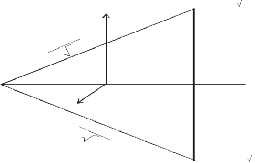
Let z - axis be taken the direction of flow along the axis of the pipe. Then u = 0, v = 0 for steady and incompressible fluid the velocity component is independent of z . The equation of continuity.
∂u + ∂v + ∂w = 0 ..................(1)
a , a 3
![]()
![]()
![]()
∂x ∂y ∂z
(a , 0)
But u = 0,
v = 0
![]()
∂w = 0......(2)
∂z
(-2a , 0)
(o, o) N x z
⇒ w = w ( x, y)........(3)
![]()
AB = BC = CA = 2a 3,
AN = 3a
B (a , - a 3 )
i.e. w is independent of z
The Navier-Stokes equations of in the absence of body forces.![]()
− ∂P = 0 ...........(4)
∂y
2 2 2
2 2 2
∂P + µ ∂ w + ∂ w − σ B0
w = 0
⇒ ∂P + µ ∂ w + ∂ w − σ B0
µ w = 0............(5)
![]()
![]()
![]()
![]()
∂z ∂ x2
∂ y 2 ρ![]()
![]()
![]()
![]()
∂z ∂ x2
∂ y 2 ρµ
2
let
![]()
σ B0
ρµ
= B2
It is clear from (3) & (4) P is independent of x & y i.e. p is the Function of z
![]()
∂p =
![]()
dp = Constant = −P
∂2 ∂2
∂z dz
∂2 ∂2
µ w +
w − B2 w = dp
⇒ w +
w − B2 w = − P .................(6)
![]()
∂x2![]()
![]()
∂y 2
dz![]()
∂x2![]()
![]()
∂y 2 µ
( D2 + D '2 − B2 ) w = − P ∴
C.F. =
a ehn x+h'n y
Where h
& h'
are related by
h 2 + h '2 − B2 = 0
![]()
µ ∑ n
P P
n n n n
∞
h x+hn y
and
![]()
P.I. = 1
![]()
![]()
− = ⇒ w (x, y) =
a e n
' + 1
P Where
h2 + h' = B2
2 2 2 2
∑ n 2 n n
D + D ' − B
µ B µ
n=1 B µ
![]()
y = x+2a
3
∞ n
![]()
P
![]()
2 an e
.......................(7)
B µ n=1
IJSER © 2015 http://www.ijser.org
International Journal of Scientific & Engineering Research, Volume 6, Issue 1, January-2015 1279
ISSN 2229-5518
∞ n
& at![]()
![]()
y = − x + 2a
⇒ ∑ an e
= − P
....................(8)
∞ hn x+h'n x+2a
3
hn x+h'n x+2a
n=1
![]()
hn x+h'n x+2a
B µ
hn x−h'n x+2a
![]()
![]()
From (7) & (8)
∑ a e
− e
3 = 0 ⇒ e
![]()
![]()
= e
n
n=1
h a+ h' a + 2ah'
h a− ah' − 2ah'
n n n n
at x
![]()
![]()
n
= a e
3 3 = e
3 3 ⇒
h' = 0,
h2 + h '2 = B2
∴ h = B
![]()
![]()
& h' = 0
n n n n n
∞ ∞ ∞
a eB x +
P = 0 ⇒
P = eBa a ⇒
a = − P
P e− Ba ⇒ w ( x, y) =
P 1 − eB ( x −a )
![]()
![]()
∑ n 2 2
![]()
∑ n ∑ n 2
![]()
1 2
n =1 B µ
B µ n =1
n =1 B µ B µ
w ( x, y) = 0
at (-2a, 0) &
w( x, y)
= 0 at
![]()
(a, a 3)
P ∞
![]()
− =
B2 µ
P ∞
∑
n=1
an e−2 ahn
...................(9)![]()
− =
B2 µ
∑
n=1
an eahn +a
![]()
3 h'n
....................(10)
ahn + a
![]()
3 h 'n = −2ahn ⇒ a![]()
3 h 'n = −3ahn ⇒
h 'n = −![]()
3 hn
h '2 + h2 = B2
⇒ 4h2 = B2
⇒ h = ± B &
h ' =
![]()
3 B , ∑ a
= − P
eBa
![]()
n n n n 2
![]()
2 n=1 n B µ
![]()
P B( x − 3 y + 2 a )

w ( x, y) =
![]()
1 − e 2
2 B2 µ
w ( x, y) = 0
at (−2a, 0) &
w( x, y)
= 0 at
(a,
![]()
− a 3)
P ∞
![]()
− =
B2 µ
P ∞
∑
n=1
an e−2ahn
....................(11)![]()
B 3 B ∞
![]()
− =
B2 µ
P Ba
∑
n=1
![]()
an eahn −a
P
3 h'n
.........................(12)![]()

B( x + 3 y + 2 a )
![]()
2
On solving: hn = ,![]()
2
h 'n =
2
& ∑ an = − B2 µ e
⇒ w3 ( x, y) = 2 1 − e
B
B( x + 2 a )
![]()
− 3 B y
n=1
B( x + 2 a )
![]()
=3 B y −
w( x, y) =
![]()
![]()
P 1 − e 2 . e
![]()
2 + e 2 e 2
− eB ( x a)
B2 µ
=B( x + 2 a )
![]()
3 B y
![]()
=3 By
= P
1 − e 2
e 2
−
+ e 2
− eB( x−a)
B2 µ
IJSER © 2015 http://www.ijser.org
International Journal of Scientific & Engineering Research, Volume 6, Issue 1, January-2015 1280
ISSN 2229-5518
![]()
w( x, y) =
P
![]()
1 − 2 Cosh
3 B y
B( x + 2 a )
![]()
e 2
− eB ( x −a )
........... (13)
B2 µ 2
![]()
B( x + 2 a )
![]()
![]()
a
Q = w ( x, y) dx dy =
3
P
![]()
1 − 2 Cosh
3 By e 2
− eB( x −a ) dx dy
∫∫ ∫ =− ∫
x 2a
B2 µ
![]()
y=− x+2a
2
3
x+2a
B( x + 2 a )
![]()
= 2P a
3 1 − 2 Cosh
3 By![]()
e 2 − eB( x −a )
dy dx
![]()
![]()
B2 µ ∫−2a ∫0 2
= 2P a
x + 2a 4![]()
![]()
−
B ( x + 2a )
![]()
Sinh e
B( x + 2 a )
![]()
2
− =x + 2a
eB( x −a ) dx
![]()
B2 µ ∫−2a
3 3 B 2![]()
3
![]()
= 1 a {eB( x+ 2 a ) −1} dx
1 eB( x+ 2 a )
![]()
![]()
=
a
− x
1 e3aB
![]()
![]()
=
− a −
1 1 e3aB
![]()
![]()
![]()
− 2a =
1
![]()
− − 3a =
![]()
1 {e3aB −1 − 3a B}
2 ∫−2a
2 B
−2a
2 B B
2 B B
2B
a B( x + 2 a )
B ( x + 2a )
a B( x + 2 a ) e
B( x + 2 a )
![]()
2
![]()
− B( x + 2 a )
− e 2![]()
Let I =
![]()
e 2 Sinh
. dx =![]()
![]()
e 2 dx
1 ∫−2a
2 ∫−2a
2
+ + a
a
Let I =
( x 2a ) B( x −a )
![]()
e dx =
1 ( x 2a )
eB( x −a )
![]()
− a 1
eB( x −a ) . dx
2 ∫−2a
![]()
3 3 B
−2a
∫−2a B
1 3a
1 { B( x−a ) }a
1 3a
1 {1
e 3aB }
1 3a 1
e−3aB
1 3a B 1
e 3aB
= − e
= − − −
= − + =
− + −
![]()
![]()
![]()
3 2 −2a
![]()
![]()
![]()
3 2
![]()
![]()
![]()
![]()
3 2 2
![]()
3 2
B B
B B
B B B B
a ( x + 2a )
( x + 2a ) a
(3a )2
9a2![]()
3 3 a2
Let I3 = ∫−2a
![]()
![]()
dx =
3 2 3![]()
![]()
= = =
2 3 2 3 2
−2a![]()
2
∴ Q =
2P I −
4 I − I
= 2P
3 3 a
−
4 . 1
{e3aB −1 − 3a B} −
1 {3a B −1 + e−3aB }
![]()
µ B2 3
![]()
![]()
3B 1 2
µ B2 2
![]()
![]()
3 B 2 B
![]()
3 B2
![]()
Q = 2P
9a2 2![]()
![]()
−
e3aB +
![]()
![]()
2 + 6a![]()
![]()
![]()
− 3a + 1 − 1
e−3aB
µ B2 2 3 3 B2
3 B2
3 B 3 B
3 B2
3 B2 ![]()
= 2P
9a2![]()
+![]()
![]()
![]()
3 + 3a − 2![]()
e3aB − 1
e−3aB
µ B2 2 3 3 B2
3 B 3 B2
3 B2
IJSER © 2015 http://www.ijser.org
International Journal of Scientific & Engineering Research, Volume 6, Issue 1, January-2015 1281
ISSN 2229-5518
Q = 2P
9a2
+ 3 (a + 1 ) −
1 (2e3aB − e−3aB )
.............. (14)![]()
![]()
3µ B2 2![]()
![]()
![]()
B B B2
Since w( x, y) =
![]()
P 3 B y
![]()
1 − 2 Cosh e
B( x + 2 a )
![]()
2
− eB( x −a )
µ B2 2
![]()
![]()
Let q = u i + v j + wk =
P
![]()
1 − 2 Cosh
3 B y
B( x + 2 a )
![]()
e 2
− eB( x −a ) k
µ B2 2
Let Ω x , Ω y
& Ω z
![]()
=B( x + 2 a )
![]()
B( x + 2 a )
![]()
∂w ∂v P![]()
![]()
![]()
x
3 B Sinh 3 B y 2![]()
![]()
3 P e 2
Sinh
3 B y
Ω = − = −
e = −
∂y ∂z
µ B2
2 µ B 2
B( x + 2 a )
B( x + 2 a )
![]()
![]()
![]()
Ω = ∂u − ∂w = − P
![]()
3 B y
−B Cosh
![]()
2 − BeB( x−a ) =
![]()
P 3 B y
![]()
Cosh
![]()
2 + eB( x−a ) &
Ω = 0
y ∂z ∂x 2 2 e
e z
µ B 2
dx
![]()
![]()
dx = dy
Ω x Ω y![]()
![]()
![]()
![]()
=![]()
= dz
Ω z
dy
![]()
= dz
3 P B( x + 2 a )
3 B y P
3 B y
B( x + 2 a ) 0
− e 2
Sinh
Cosh e 2
+ eB( x −a )
µ B
Taking I st
Two
2 µ B 2 ![]()
![]()
dx = dy
− 3 e![]()
B( x + 2 a )
2
Sinh
3 B y
Cosh
3 By
B( x + 2 a )
![]()
e 2
+ eB( x −a )
![]()
Cosh 3 B y
2
B( x + 2 a )
![]()
2
2
+ eB( x −a )
2 ![]()
3 B y
B( x + 2 a )
dx +
![]()
3 ∫ Sinh 2
dy = C1
![]()
e 2
![]()
![]()
B( 2 x −2 a − x −2 a )
![]()
∫ Cosh
3 B y dx + ∫
e 2 dx + 3 .
2 Cosh
3 B y
= C
2
B ( x + 2a )
∫ Cosh dx +
B( x −4 a )
![]()
∫ e 2
dx +
![]()
3 B 2 1![]()
2 Cosh 3 B y = C
2 Sinh
![]()
2
B ( x + 2a ) 2
![]()
![]()
+
B( x −4 a )
![]()
e 2
![]()
B
![]()
+ 2 Cosh 3 B y = C
2
⇒ Sinh
1
B ( x + 2a )
B( x −4 a )
![]()
+ e 2
+ Cosh
![]()
3 B y
C B
= 1 = A
![]()
B 2 B B
![]()
![]()
2 1 2 2 2
IJSER © 2015 http://www.ijser.org
International Journal of Scientific & Engineering Research, Volume 6, Issue 1, January-2015 1282
ISSN 2229-5518
B( x −4 a )
![]()
![]()
B y B y
The first vortex line![]()
e 2 + Sinh 3
![]()
![]()
+ Cosh 3
= A ................... (15)
taking last two
dz = 0
2 2
⇒ the second vortex line z = B
2
.................. (16)
Let P = 2 ,
µ = .5 ,
are fixed and B =
![]()
σ B0 , ( x, y ) are change
ρµ
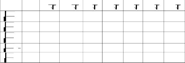
( x, y )
−9, 1
−12 , 1
−15 , 1
−18 , 2
−21, 3
−24 , 4
−27 , 5
6 3
σ B0
ρ µ
σ B0
ρ µ
σ B0
ρ µ
σ B0
ρ µ
σ B0
ρ µ
= 1
= 1
2
= 1
3
= 1
4
= 1
6
w ( x, y ) w ( x, y ) w ( x, y ) w ( x, y )
w ( x, y )
2 3
3
3
3
3 3
In this paper, we have investigated the velocity
w( x, y) by the table-1 of equation (13) between
velocity and point ( x, y) , it is clear that the
[1] Chernyshenko S. I. (1982), an approximate method of determining the vorticity in the separation region as the viscosity tends to zero. Fluid Dynamics .17 pp 1-11.
velocity
w( x, y) of increases in the interval
[2] Cherukat P., Mclaughlin J. B. & Graham A.
− 9 ,
1
≤ ( x, y ) ≤ − 27 ,
5 at the different
L. (1994), the inertial lift on a rigid sphere![]()
![]()
![]()
6 3 3
2
translating in a linear shear flow fluid. Int. J.
Multiphase flow vol. 20, No. 2, pp 339-353.
values of
σ B0
ρµ
. Again the velocity
w( x, y)
[3] Chida K. (1983), Heat transfer in steady laminar pipe flow with liquid solidification.![]()
increases correspondingly in the interval
2
Heat Transfer: Jap. Res. 81, pp 81–94.
[4] Chikh S., Boumedien A., Bouhadef K. &
− 9 ,
1
≤ ( x, y ) ≤ − 27 ,
5 when
σ B0
Lauriat G. (1995), Analytical solution of![]()
![]()
6 3
3
ρµ non-Darcian forced convection in an annular
![]()
decreases from1 to 1 . Negative sign of velocity
6
w( x, y) shows that the direction of flow is in opposite to the direction of motion of fluid. Also we have investigated the volumetric flow, vortex lines respectively by the equations (14), (15) & (16).
duct partially filled with a porous medium. Int. J. of Heat Mass Transfer, Vol. 38, pp
1543-1551.
[5] Childress S. (1966), Solutions of Euler’s
equations containing finite eddies. Phys. Fluids 9 pp 860–872.
[6] Chongsheng C., Mohammad A. R. & Edriss
S.T. (1999), The Navier-Stokes Equations
on the rotating 2-D sphere: Gevrey relularity
IJSER © 2015 http://www.ijser.org
International Journal of Scientific & Engineering Research, Volume 6, Issue 1, January-2015 1283
ISSN 2229-5518
and asymptotic degrees of freedom. Z. angew. Math. Phys. 50, pp 341-360.
[7] Chukkapali G. & Turan Q. F. (1995), Structural parameters and Prediction of
[8] Cumber batch E. & Wu T. Y. (1961), Cavity flow past a slender hydrofoil. Private
communication. J. Fluid Mech.11, pp 187–
208.
[9] Dauchot O.,. Daviaud F., Hegseth J. & Berge P. (1992), Subcritical transition to turbulence in plane Couette flow. Phys. Rev. Lett. 69, pp
2511–2514.
[10] De. U.S. (1994), Importance of mountain waves in aviation and weather Hazzard associated with it. Proc. Indian Natn. Sci. Acad 60 A. No. 1, pp 217-226.
[11] Dennis S. C. R. & Chang G-Z. (1970), numerical solutions for steady flow past a circular cylinder at Reynolds numbers up to
100. J. fluid mechanics 42, pp 471-489.
.
adverse pressure gradient Turbulent Flows an Improved K.F. Model. J. of Fluids Engng. Vol. 117, No.3, pp 424-432.
[12] Dennis S. C. R., Ng M. & Nguyen P. (1993), Numerical solution for the steady motion of a viscous fluid inside a circular boundary using integral conditions. J. Comput. Phys. 108 pp 142–152.
[13] Ding Y. & Kawahara M. (1998), linear
stability of incompressible fluid flow in a cavity using finite element method. Int. j. for numerical methods in fluids 27, pp
139-157.
[14] Dubey R. K. & Sharma R. G. (1978), A Note on the flow of Visco-elastic fluids through a rectilinear Pipe having its cross section as a parallelogram with pressure gradient as any function of time. Reprinted from Def. Sci. J. vol. 28, No.3, pp 341-
360.
IJSER © 2015 http://www.ijser.org