International Journal of Scientific & Engineering Research, Volume 5, Issue 7, July-2014 216
ISSN 2229-5518
Stability analysis of prey-predator model with alternative food sources and transition two
diseases in the same population
Rasha Majeed Yaseen
Department of Mechatronics, Al-Khwarizmi College of Engineering, University of Baghdad / Iraq.
E-mail addresses: rasha.majeed1@gmail.com
Diseases in a prey-predator system have received significant interest in resent years. It is well known that, in nature species does not exist alone. In fact, any given habitat may contain dozens or hundreds of species, some times thousands. Since![]()
dP = P(a − bP) − cP−
dT
![]()
d− = −(ecP − θ )
dT
(1)
any species has at least the potential to interact with any other
where
P(T )
and
−(T )
represent the densities of prey and
species in its habitat, the possibility of spread of the disease in
a community rapidly becomes astronomical as the number of
infected species in the habitat increases. Therefore, it is more
predator species at time T respectively. Clearly the above model is a simple Lotka-Volterra prey-predator model with logistic growth rate for prey. The positive parameters
of biological significance to study the effect of disease on the
dynamical behavior of interacting species
a , b , c , e
and θ represent intrinsic growth rate, intra-specific
many researchers, especially in the last two decades, have proposed and studied different prey-predator models in the presence of disease in one of the species see for example [1-13] and the references there in. In most previous studies, the only means of transmission of disease is the direct contact
competition, attack rate, conversion rate and natural death
rate respectively [16].
We impose the following assumptions:
2.1 In the presence of first disease, SIS disease, the predator
population consists of two subclasses, namely, the susceptible
between individuals. However, many diseases are transmitted
predator S(T )
and the infected predator by this disease I1 (T ) .
in the species not only through contact, but also directly from environment.
2.2 In the presence of second disease, SI disease, the predator
population consists of two subclasses, namely, the susceptible
Elisa Elena et al [14] proposed prey-predator model two
predator S(T )
and the infected predator by this disease I 2 (T ) .
diseases affect the prey. Predators are allowed to have other food sources. Fabio Roman et al [15] proposed prey-predator model containing two disease strains in the predator population.
On contrast to all of the above studies, in this paper a
Therefore at any time T we have −(T ) = S(T ) + I1 (T ) + I 2 (T ) .
2.3 The susceptible predator has an alternative food sources supplied by a constant rate β > 0 .
2.4 Both of the diseases, SIS and SI, transmitted among the predator individuals only, but not the prey individuals, by
prey-predator model involving SIS and SI infectious diseases
in predator species is proposed and analyzed. It is assumed that the predator population has external source of food. It is
contact with an infected predator at infection rate α1 > 0
α 2 > 0 respectively.
and
assumed that both of the diseases spread within predator
2.5 Only the first disease disappears and the infected predator
population by contact between susceptible individuals and
becomes susceptible predator again at a recover rate
w > 0 .
infected individuals. Further, in this model, linear type of functional response as well as linear incidence rate for describing the transition both of disease are used.
The basic prey-predator model is
Finally both of the diseases, SIS and SI, induces the mortality
within the infected predator individuals at a constant rate
δ1 > 0 and δ 2 > 0 .
2.6 The infected predator, by SIS disease, feed on the prey species according to Lotka-Volterra functional response with attack rate constant τ 1 > 0 . Also, the infected predator by SI disease feed on the prey species by functional response with attack rate constant τ 2 > 0 .
IJSER © 2014 http://www.ijser.org
International Journal of Scientific & Engineering Research, Volume 5, Issue 7, July-2014 217
ISSN 2229-5518
These assumptions can be mathematically realized into the following four differential equations![]()
dP = P[(a − bP) − cS − cτ I − cτ I ]
dT 1 1 2 2
Now, by using Gronwall lemma [17], it obtains that:![]()
0 < Μ(t ) ≤ Μ(0)e−φ t + π (1 − e−φ t )
φ
π
![]()
= S(ecP − α1I1 − α2 I2 − θ + β ) + wI1![]()
which yields lim sup Μ(t ) ≤
t →∞ φ
that is independent of the initial
dT
![]()
dI1
dT
= I1(ecτ 1P + α1S − θ − δ 1 − w)
(2)
conditions. ■
The system (3) has at most eleven biologically feasible![]()
dI2
equilibrium points, namely E
= (p
, s , y
, y ), k = 0,1,2, ... ,10 .
= I2 (ecτ 2 P + α2S − θ − δ 2 )
k k k 1k 2 k
dT
In order to simplifying the proposed model (2), the following
The existence conditions for each of these equilibrium points are discussed in the following:
dimensionless variables are used:
3.1 The vanishing equilibrium point
E = (0 , 0 , 0, 0)
always![]()
t = aT , p = c P,
a
![]()
s = c S,
a
![]()
c y1 =
a
I1 ,
c
![]()
y2 = I 2
a
exists.
E = (0, s , 0 , 0)
Thus we obtain the following dimensionless form of the model
(3):
1
where s1 is any positive number, exists if and only if
1
h4 = 0 .
dp = p[(1 − h p) − s − τ y
− τ y ]
![]()
dt 1
ds
1 1 2 2
E2 = (p2 , 0 ,0, 0) where p2 = 1![]() h1 , always exists.
h1 , always exists.
3.4 The first disease and prey free equilibrium point![]()
= s(ep − h2 y1 − h3 y2 + h4 ) + h5 y1
dt
(3)
E3 = (0 , s3 , 0 , y2 3 ) where:![]()
dy1
= y1(eτ 1p + h2 s − h5 − h6 )
h 7 h 4
![]()
![]()
dt s3 = and y2 3 = (4)
![]()
dy2
h 3 h 3
= y2 (eτ 2 p + h3s − h7 )
dt
exists uniquely in the interior of the first quadrant of
Where:
s y2 − plane under the following necessary and sufficient
b h1 =
α1
![]()
> 0, h2 =
α2
![]()
> 0, h3 =
> 0, h4 =![]()
β − θ
∈ ℜ,
condition
h 4 > 0 .
a
![]()
h = w > 0, h
c c
![]()
= θ + δ1 > 0, h
a
![]()
= θ + δ 2 > 0
3.5 The second disease and prey free equilibrium point
E4 = (0 , s4 , y14 , 0) where:
5 c 6 a 7 a
represent the dimensionless parameters of the model (2). The
h 5 + h 6
![]()
s =
and y
h 4 (h 5 + h 6 )
![]()
=
(5)
4
initial condition for model (3) may be taken as any point in 2
h 2 h 6
the region ℜ4 . Obviously, the interaction functions in the right hand side of system (3) are continuously differentiable
exists uniquely in the interior of the first quadrant of
s y1 − plane under the following necessary and sufficient
functions on ℜ4 , hence they are Lipschitizian. Therefore the
condition
h 4 > 0 .
solution of system (3) exists and is unique. Further, all the
3.6 The first disease and susceptible predator free equilibrium
solutions of system (3) with non-negative initial condition are
point E = (p
, 0 , 0 , y2 5
) where:
uniformly bounded as shown in the following theorem.
h 7 e τ 2
− h 1 h 7
![]()
p5 =
e τ
![]()
and y2 5 =
e τ 2
(6)
in ℜ4
2 2
are uniformly bounded if the sufficient condition
+ exists uniquely in the interior of the first quadrant of
h4 < 0 holds.
p y2
− plane under the following necessary and sufficient
condition
e τ 2
> h 1 h 7 .
![]()
dp ≤ p(1 − h p)
3.7 The disease free equilibrium point E = (p
, s , 0 , 0) where:
dt 1
6 6 6
Clearly by solving the above differential inequality we get
−h 4![]()
p6 =
and s6
= 1 − h 1p 6
(7)![]()
lim sup p(t ) ≤ 1
t →∞ h1
1 1 1
e
exists uniquely in the interior of the first quadrant of
ps − plane under the following necessary and sufficient
Define the function
Μ(t ) = p(t ) +
![]()
s(t ) +
e
![]()
y1 (t ) +
e
![]()
y2 (t )
e
and
conditions
h 4 < 0
and
1 > h 1 p 6 .
then take its time derivative along the solution of system (3),
3.8 The second disease free equilibrium point
gives
E = (p
, s , y
, 0) where:
dΜ ≤ p − φ s − φ y
− φ y
where φ = min{− h , h , h }
7 7 7 17
dt e
![]()
![]()
![]()
![]()
e 1 e 2
4 6 7
h 5 + h 6 − eτ 1p7
![]()
s =
and y
(h + h − eτ p )(ep + h )
![]()
= 5 6 1 7 7 4
(8)
≤ π − φ Μ
where![]()
π = (1 + φ ) 1
H
7
2
IJSER © 2014 http://www.ijser.org
17 (h
− eτ 1p 7 )
International Journal of Scientific & Engineering Research, Volume 5, Issue 7, July-2014 218
ISSN 2229-5518
while p7
represents a positive root of the following second
β11 = 1 − 2h 1p − s − τ 1y1 − τ 2 y2 ,
β12 = −p ,
β13 = −τ 1p ,
order polynomial equation
2
β14
= −τ 2 p ,
β2 1
= es , β2 2
= ep − h
2 y1
− h 3 y2
+ h 4 ,
A1p
+ A2 p + A3 = 0
β = −h s + h , β
= −h s , β
= eτ y , β
= h y ,
where
2 3 2 5 2 4 3
31 1 1 3 2 2 1
A1 = e τ 1 h 1 h 2 > 0 ;
β3 3 = eτ 1p + h 2 s − h 5 − h 6 ,
β3 4 = 0 ,
β4 1 = eτ 2 y2 ,
A = − (h h
h + eτ h − eτ (h + τ h
));
β4 2 = h 3 y2 ,
β4 3 = 0 ,
β4 4 = eτ 2 p + h 3s − h 7
2 1
A3 = h 2 h 6
2 6
− (h
1
+ h 6
2
)(h
1 6 1 4
+ τ 1 h );
In what follows, the system’s equilibria are
[k ]
Ek and we denote
Therefore, straight forward computation shows that E7
exists
by J k
Ek i =
and
βi j
j =
the Jacobian and its entries evaluated at
k =
uniquely in the interior of the first octant of
ps y 1 − plane if
, 1,... ,4 ,
1,... ,4 ,
0,1,2,... ,10
and only if the following conditions are hold.
e p > −h
, h > max{eτ p
, τ h }
and
The equilibria E0
is saddle point, since its eigenvalues are
7 4
h h < (h
6 1 7 1 4
+ h )(h + τ h )
1 > 0 , h 4 , − (h 5 + h 6 )< 0 and −h 7 < 0 .
2 6 5
6 6 1 4
3.9 The first disease free equilibrium point
where:
E = (p
, s8
, 0 , y2 8 )
E1 is
p8 =
h 3− h 7 − τ 2 h 4
![]()
,
s8 =
![]()
h 7 − eτ 2 p8
![]()
and y = e p8 + h 4 (9)
1 − h1 p < s1
< min
s ,
h 7 h 6 s
![]()
![]()
,
(10)
h 1h 3 h 3 h 3
h 3
h 2 s − h 5
exists uniquely in the interior of the first octant of ps y2 − plane
under the following necessary and sufficient conditions
h 7 V [1] = p +
![]()
![]()
1 s − s − s ln s ![]()
![]()
y1 + y2
![]()
h 4 > 0 , p8 <
eτ
and
h 3 > h 7 + τ 2 h 4 .
e 1
s1 e e
3.10 The prey free equilibrium point E = (0 , s
, y19
, y2 9
) where:
Clearly,
V [1] :
ℜ4 → ℜ
and
V [1] (E ) = 0
with
s = h 5+ h 6 = h 7
and y
(h + h )(h − h y )
= 5 6 4 3 2 9
where
y is
V [1] (E) ≠ 0
∀ E ≠ E1
, E ∈ ℜ4 . Hence it is positive definite![]()
![]()
9 h h
![]()
19 h h
2 9 function in ℜ4
. Also, the derivative of V [1] with respect to the
2 3 2 6
+
time t is given as follows.
any positive number,
E9 exists uniquely in the interior of the
[1]
first octant of
s y1 y2 − plane under the following necessary
![]()
dV = p(1 − h p − s )+ y1 h s − h5 s − h
and sufficient conditions
h (h
5+ h
)= h
2 h 7 ,
h 4 > 0
and
dt 1
h 4
1 e 2 1 s 1 6
y2
h 4 > h 3 y 2 9 .
E = (p
, s , y
, y )
+ (s − s1 ) +
e
![]()
(h s − h )
e
where
10 10 10
110
2 10
Since E1 exists if and only if h 4 = 0 , in addition condition (10),
[1]
h 2 h 7
− h (h
5+ h 6
τ (h
5+ h
)− τ h
guarantee that![]()
dV < 0
on subregion of
ℜ4 , then
V [1]
is a
p10 =
![]()
e(τ h
2 − τ 1h 3
; s10 =![]()
(τ h
;
2 − τ 1h 3
dt
Lyapunov function on that subregion which satisfy condition
[1]
![]()
y = 1 [1 − h p
− s − τ y ]
(10). since![]()
dV < 0
on subregion of ℜ4
then
E is a locally
210
2
1 10 10
1 110
dt + 1
s10
[e(τ h
2 + τ 1h
)(h
+ τ 2 h
4 − h
)+ h h
(h h
− h (h
5+ h
))]
asymptotically stable but not globally. ■
y110 =
![]()
e(τ h
6 − τ 1h
)(τ h
2 − τ 1h 3
4
E2 is locally
Therefore, straight forward computation shows that E10 exists
asymptotically stable in ℜ+ if and only if:
uniquely in the Int. ℜ4
if and only if the following conditions
< − h5 + h6
h 7
+
are hold.
ep2
![]()
min
h4 ,
1
![]()
,
τ 2
(11)
max
h (h
![]()
5+ h
6 , h
− τ 2 h 4
< h 7![]()
< τ 2 h 6
; τ 2 h
2 > τ 1h 3
and
is given
h 2
τ 1
by:
1 − 2h p −p
−τ p
−τ p
1 > h 1p10 + s10 + τ 1y110
The Jacobian matrix of system (3) is
J = (βi j ) ∈ ℜ4 x 4 , with
J2 =
1 2 2 1 2
0 ep2 + h 4 h 5
− −
2 2
0
entries
0 0
eτ 1p2 h 5 h 6
0
0
eτ 2 p2 7
So, the characteristic equation of J 2 can be written by
(1 − 2h p
− µ )(ep + h
− µ )(eτ p − h − h − µ )×
1
(eτ p
2
2 − h
p 2
7 − µy 2
4
)= 0
s 1 2 5 6 y1
IJSER © 2014 http://www.ijser.org
International Journal of Scientific & Engineering Research, Volume 5, Issue 7, July-2014 219
ISSN 2229-5518
from which, we obtain that:
dV [ 4]
= p(1 − h p − s
− τ y
)+ h 4 (s − s ) + h6 (y − y )
µp = 1 − 2h1p2 < 0
, µs = ep2 + h 4 , µy1 = eτ 1p2 − h 5 − h 6
and![]()
dt 1
![]()
![]()
4 1 14 e
4 e 1 14
µy2 = eτ 2 p2 − h 7
y2
![]()
3 4 − h 7
![]()
)+ s 4 y1 (h s − h
![]()
)+ y14 (h
− h s)
Here
µp , µs , µy1
and
µy 2 denote to the eigenvalues in the
e es e
[ 4 ]
p − direction,
s − direction,
y1 − direction and
y2 − direction,
Hence,![]()
dV < 0
on subregion of ℜ4
under the sufficient
respectively. So, it is easy to verify that, all the eigenvalues have negative real parts if and only if the condition (11) holds.
dt
condition (13), then
4
V [ 4 ]
is a Lyapunov function on that
Therefore, the equilibrium point E2
is locally asymptotically
subregion of ℜ+
which satisfies condition (13). Therefore E4
stable in
ℜ4 . Furthermore, it is a globally asymptotically
is a locally asymptotically stable but not globally. ■
stable too. ■
E5 = (p5 , 0 , 0 , y2 5 )
is locally asymptotically stable in ℜ4 if and
E = (0 , s , 0 , y
) is locally asymptotically stable in ℜ4
if and
only if:
3
only if:
3 2 3
(h + τ 2 h 4 )
h 5h 7
+
h 6![]()
h 3 y2 5 < h 4 , p < p5 < min
eτ 1
(h y − h )
![]()
,
e
(14)![]()
1 − h1p <
h
![]()
, s < (h h
− h h )
and
h 2 h 7 > h 3 h 6
(12)
and
1 − h p < τ y
3 2 7 3 6
1 2 2 5
p s y 1 y
V [ 3] = p + 1 s − s
− s ln s + y1 + =1 y − y
− y ln y2
[ 5]
1
2
![]()
e 3
![]()
![]()
s3 e
![]()
2 3 2 3
y2 3
V = p − p5 − p5 ln
![]()
![]()
+ +
5 e
+ y2 − y2 5 − y2 5 ln
y
2 5
Clearly,
V [ 3]
: ℜ+ → ℜ
and
V [ 3]
(E3 ) = 0
with
Clearly,
V [ 5]
: ℜ+ → ℜ
and
V [ 5]
(E5 ) = 0
with
V [ 3] (E) ≠ 0
∀ E ≠ E3
, E ∈ ℜ4 . Hence it is positive definite
V [ 5] (E) ≠ 0
∀ E ≠ E5
, E ∈ ℜ4 . Hence it is positive definite
function in ℜ4 . Also, the derivative of V [ 3] with respect to the
function in 4
[ 5]
+
time t is given as follows.
[ 3]
ℜ+ . Also, the derivative of V with respect to the
time t is given as follows.
[ 5]
dV
h 7 τ 2 h 4
![]()
![]()
y1 h 2 h 7
h5h 7
![]()
dV = p(1 − h p − τ y
h 4![]()
s + p
![]()
− h 3 y2 5
+ y τ h![]()
− h6 ![]()
= p 1
dt
![]()
− h 1p −
h
![]()
− +
h
e h
− h6![]()
−
h s
dt 1
2 2 5
5 1 1 5
[ 3]
3 3 3 3
+ h 1 p5 (p − p5 )
Hence,![]()
dV < 0
dt
on subregion of 4
under the sufficient
Hence,
dV [ 5]
![]()
< 0
on subregion of 4
under the sufficient
condition (12), then
V [ 3]
is a Lyapunov function on that dt
subregion of ℜ4
which satisfies condition (12). Therefore E3
condition (14), then
V [ 5]
is a Lyapunov function on that
is a locally asymptotically stable but not globally. ■
subregion of ℜ4
which satisfies condition (14). Therefore E5
is a locally asymptotically stable but not globally. ■
point E = (0 , s , y
, 0) is locally asymptotically stable in ℜ4 if
4
and only if:
4 14
E6 = (p6 , s6 , 0 , 0) is locally asymptotically stable in ℜ+
only if:
if and
h 2 h 6
(1 − h p)< (h
+ h 6
)(h
+ τ 1h 4
) , y
< y14 ,
h 7
![]()
s 4 <
h 3
p < p s <
h 7 ![]()
y
h 5
![]()
and s <
(15)
and
h 6
y1 < s < s 4 ,
(13)
6 , 6
minτ 1
1 ,
h 3 h 2
![]()
V [6 ]
= p − p6
p
![]()
− p ln +![]()
1 s − s
s y y
![]()
![]()
![]()
− s ln + 1 + 2
p6 e
s6 e e
![]()
V [ 4 ] = p + 1 s − s
− s ln![]()
s + =1 y − y![]()
![]()
− y ln y1 + 1 y
[6 ] 4
[6 ]
4 4
ps4
14 2
14
Clearly,
V : ℜ+ → ℜ
and
V (E6 ) = 0
with
Clearly,
V [ 4 ]
: ℜ4 → ℜ
and
V [ 4 ]
(E4 ) = 0
with
V [6] (E) ≠ 0
∀ E ≠ E6
, E ∈ ℜ4 . Hence it is positive definite
V [ 4] (E) ≠ 0
∀ E ≠ E4
, E ∈ ℜ4 . Hence it is positive definite
function in ℜ4 . Also, the derivative of V [6 ] with respect to the
time t is given as follows.
function in ℜ4 . Also, the derivative of V [ 4 ] with respect to the
time t is given as follows.![]()
dV [6]
= (p − p )(1 − h p)+ p (s
− τ y![]()
)+ s 6 y1
(h s − h )
dt 6
y
1 6 6
h
1 16 e s
![]()
+ 2 (h s![]()
− h )− y
+ p s
+ 2s p
+ τ p y
e 3 6 e 6
6 2 6 2
IJSER © 2014 http://www.ijser.org
International Journal of Scientific & Engineering Research, Volume 5, Issue 7, July-2014 220
ISSN 2229-5518
Hence,
dV [6 ]
![]()
< 0
on subregion of 4
under the sufficient
Hence,
dV [8 ]
![]()
< 0
on subregion of 4
under the sufficient
dt
condition (15), then
V [6 ]
is a Lyapunov function on that
dt
condition (17), then
V [8 ]
is a Lyapunov function on that
subregion of ℜ4
which satisfies condition (15). Therefore E6
subregion of ℜ4
which satisfies condition (17). Therefore E8
is a locally asymptotically stable but not globally. ■
is a locally asymptotically stable but not globally. ■
E = (0 , s , y
, y ) is
E = (p
, s , y
, 0) is
locally asymptotically stable in 4
9 9 19 2 8
7 7 7 17
ℜ+ if and only if:
locally asymptotically stable in ℜ4 if and only if:
1 − h p < s
+ τ y
+ τ y
, y >
h 4 h 5
eτ 2 p7 + h 3s7 < h 7 , s < (h
+ h )y
h 5 s7 y1
![]()
+ (h y
− h )s
and p < p7
(16)
1 9 1 19
2 2 9
![]()
2 9 h (h
+ h 6 )
(18)
5 6 17
2 1 4 7
h 6 h 7 y 2 9
and
![]()
h (h
− h 3 y 2 9
) < s < s9
V [7 ] = p − p
− p ln + s − s
− s ln s
![]()
![]()
7 7
p7
![]()
7 7
7
s y ![]()
9
− s9
1![]()
![]()
ln + y1
− y19
− y19![]()
ln 1
+ =1 y − y − y ln
1 17 17
![]()
![]()
y1 + y2
y17 e
e s9 e
y19
+ =1 y − y
y
− y ln
Clearly,
V [7 ]
: ℜ+ → ℜ
and
V [7 ]
(E7 ) = 0
with
2 2 9
![]()
2 9 y
2 9
V [7 ] (E) ≠ 0
∀ E ≠ E7
, E ∈ ℜ4 . Hence it is positive definite
Clearly,
V [9 ]
: ℜ4 → ℜ
and
V [9 ]
(E9 ) = 0
with
function in ℜ4 . Also, the derivative of V [7 ] with respect to the
[9] ( ) 4
+
time t is given as follows.
V E ≠ 0
∀ E ≠ E9
, E ∈ ℜ+
. Hence it is positive definite![]()
dV [7 ]
h![]()
4
7 1 7
![]()
− h 2 y
17
− p s 7 + τ 1 y17
function in ℜ4 . Also, the derivative of V [9 ] with respect to the
time t is given as follows.
dt
=h
e e
h 3 h 7
![]()
dV [9 ]
= p(1 − h p − s − τ y − τ y )+
1 h5s
![]()
![]()
(h y − h )+ h y
+ y τ p −
6 + y
τ p + s − dt
e h6
1 1 7 e
![]()
![]()
2 2 7 7
h y ( ) (h
+ h ) (
( ))
+ (h 5 + h 6 )
+ (h y − h )s
h
![]()
− s 7 y1
![]()
+ 5 1
s − s 9 +
h4 h5 − h3 y2 9 h5 + h6
2 6
![]()
17
e
[7 ]
7 5
![]()
e es
Since
es eh h
E9 exists if and only if
h 4 > h 3 y2 9 , in addition
Hence,![]()
dV < 0
dt
on subregion of 4
under the sufficient
condition(18) guarantee that
dV [9 ]
![]()
< 0
dt
on subregion of
ℜ4 ,
condition (16), then
V [7 ]
is a Lyapunov function on that
then
V [9 ]
is a Lyapunov function on that subregion which
subregion of ℜ4
which satisfies condition (16). Therefore E7
satisfies condition (18). Therefore
E9 is a locally
is a locally asymptotically stable but not globally. ■
asymptotically stable but not globally. ■
E = (p
, s , 0 , y
) is
E is
8 8 8 2 8 10
locally asymptotically stable in ℜ4 if and only if:
locally asymptotically stable in ℜ4 if and only if:
eτ p
+ h s < h
, es p (h
+ τ h
)< h (h
− eτ p ) and p < p
(17)
h −h h
1 8 2 8 6
8 7 2 4
5 7 2 8
![]()
max τ ,![]()
τ , < p < p 10 , s + τ 1 y 1 + τ 2 y2 < 1 − h 1 p ,
e 1
e e 2
[8]
![]()
![]()
![]()
![]()
1
s y
2 10
h 5
V = p − p8 − p8 ln +
s − s8 − s8 ln +![]()
y2 < miny2 10 ,
![]()
s < mins 10 ,
(19)
p8 e
s8 e
s 10
s y
h 2
+ =1 y − y
y
![]()
− y ln
and
![]()
110 < y < y
2 2 8
2 8 y
2 8
s 10
1 110
Clearly,
V [8 ]
: ℜ+ → ℜ
and
V [8 ]
(E8 ) = 0
with
V [8 ] (E) ≠ 0
∀ E ≠ E8
, E ∈ ℜ4 . Hence it is positive definite
V [10] = s −
p10
![]()
![]()
− p10 ln
s10
![]()
− s10 ln
function in ℜ4 . Also, the derivative of V [8 ] with respect to the
p10 e
s10
time t is given as follows.
+ =1 y − y
− y ln![]()
y1 + =1 y − y
− y ln![]()
y2
[8]
1 110
110
2
2 10
2 10
![]()
dV = (p − p )(1 − h p)− p(s
+ τ y
)+ y τ p
+ h2 s
− h6 e
y110 e
y2 10
dt 8 1
8 2 2 8
1 1 8
e 8 e
+ (s(h y
− h s
)− h s y )
7 2 8 4 8
5 8 1
IJSER © 2014 http://www.ijser.org
International Journal of Scientific & Engineering Research, Volume 5, Issue 7, July-2014 221
ISSN 2229-5518
Clearly,
V [10 ]
: ℜ+ → ℜ
and
V [10 ]
(E10
) = 0
with
the system (3) approaches asymptotically to the equilibrium
V [10 ] (E) ≠ 0
∀ E ≠ E10
, E ∈ ℜ4 . Hence it is positive definite
point E2 = ( 0.02 , 0 , 0 , 0 ) as show as in Fig.(2).
function in
ℜ4 . Also, the derivative of
V [10]
with respect to
the time t is given as follows.
[10]
dV
![]()
= p10
dt
− p)[− (1 − h p)+ s + τ y
+ τ 2
y ]+ (ep + h
)(s − s )
+ (eτ p − h
)(y
− y2 10
)+ (eτ p − h
)(y
− y110 )![]()
+ 1 (s
y − s y
)(h s − h ) + h (s
y − s y )
s 10 1
110 2
5 3 10 2
2 10
Since
E10
exists if and only if
[10 ]
h 4 > h 3 y2 9 , in addition
condition(19) guarantee that![]()
dV < 0
dt
on subregion of
ℜ4 ,
Fig.(2): time series of the trajectories of the system (3)
which shows E2 is a globally asymptotically stable point.
then
V [10] is a Lyapunov function on that subregion which
satisfies condition (19). Therefore
E10
is a locally
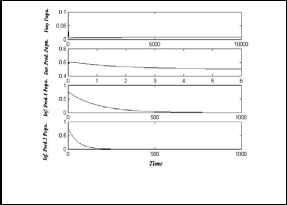
Now to show the stable of first disease and prey free
asymptotically stable but not globally. ■
equilibrium point E3
parameters values:
used the following set of hypothetical
We give some numerical analysis in support our theoretical
findings. The system (3) is solved numerically, for different sets of parameters, using predictor-corrector method with six
h 1 = 50 , h 2 = 0.8 , h 3 = 0.1 , h 4 = 0.2 , h 5 = 0.2 ,
h 6 = 0.08 , h 7 = 0.03 , e = 0.8 , τ 1 = 0.3 , τ 2 = 0.9
(22)
order Runge-Kutta method, and then the time series for the trajectories of system (3) are draw. Now before we go farther with numerical analysis, We will use the solid line (ـــــــ) for p ,
In Fig.(3), the system (3) approaches asymptotically to the equilibrium point E3 = ( 0 , 0.295 , 0 , 2.018 ) .
dash line (ــــ
ـــ) for s , dot line (….) for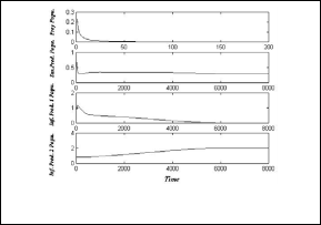
y1 , dash-dot line (ـــ .
ـــ) for y2 and the initial point ( 0.75 , 0.75 , 0.75 , 0.75 ) . in the all
of the following figures.
Now to show the stable of axial equilibrium point on the s -
axis
E1 used the following set of hypothetical parameters
values:
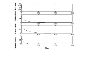
h 1 = 50 , h 2 = 0.01 , h 3 = 0.01 , h 4 = 0 , h 5 = 0.08 ,
h 6 = 0.1 , h 7 = 0.5 , e = 0.4 , τ 1 = 0.3 , τ 2 = 0.1
(20)
In Fig.(1), the system (3) approaches asymptotically to the
Fig.(3): time series of the trajectories of the system (3)
equilibrium point E1
= (0 ,1.059 , 0 , 0 ) .
which shows E3 is a locally asymptotically stable point.
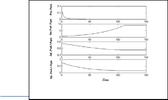
Now to show the stable of second disease and prey free
equilibrium point E4
parameters values:
used the following set of hypothetical
h 1 = 50 , h 2 = 0.8 , h 3 = 0.1 , h 4 = 0.2 , h 5 = 0.2 ,
h 6 = 0.08 , h 7 = 0.2 , e = 0.8 , τ 1 = 0.8 , τ 2 = 0.9
(23)
In Fig.(4), the system (3) approaches asymptotically to the
stable equilibrium point E4
= (0 , 0.35 , 0.875 , 0)
Fig.(1): time series of the trajectories of the system (3)
which shows E1 is a locally asymptotically stable point.
Now to show the stable of axial equilibrium point on the p -
axis equilibrium point E2
used the following set of
hypothetical parameters values:
h 1 = 50 , h 2 = 0.01 , h 3 = 0.01 , h 4 = −0.04 , h 5 = 0.08 ,
h 6 = 0.1 , h 7 = 0.5 , e = 0.4 , τ 1 = 0.3 , τ 2 = 0.1
(21)
IJSER © 20 http://www.ijser
International Journal of Scientific & Engineering Research, Volume 5, Issue 7, July-2014 222
ISSN 2229-5518
Now to show the stable of first disease and susceptible
predator free equilibrium point E5
hypothetical parameters values:
used the following set of
h 1 = 50 , h 2 = 0.8 , h 3 = 0.1 , h 4 = −0.01 , h 5 = 0.2 ,
h 6 = 0.08 , h 7 = 0.01 , e = 0.8 , τ 1 = 0.8 , τ 2 = 0.9
(24)
In Fig.(5), the system (3) approaches asymptotically to the
Now to show the stable of first disease free equilibrium point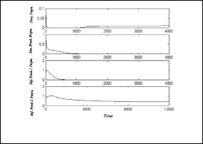
stable equilibrium point E5
= ( 0.014 , 0 , 0 , 0.385 )
E8 used the following set of hypothetical parameters values:
h 1 = 50 , h 2 = 0.5 , h 3 = 0.3 , h 4 = 0.1 , h 5 = 0.1 ,
h 6 = 0.2 , h 7 = 0.1 , e = 0.1 , τ 1 = 0.1 , τ 2 = 0.2
(27)
As shown as in Fig.(8),the system (3) approaches asymptotically to the equilibrium point
E = ( 0.013 , 0.332 ,0 , 0.342 ) .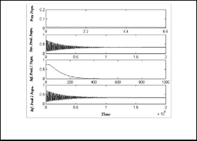
Fig.(5): time series of the trajectories of the system (3)
which shows
E5 is a locally asymptotically stable point.
Now to show the stable of disease free equilibrium point E6
used the following set of hypothetical parameters values:
h 1 = 50 , h 2 = 0.1 , h 3 = 0.2 , h 4 = −0.001 , h 5 = 0.08 ,
h 6 = 0.1 , h 7 = 0.5 , e = 0.4 , τ 1 = 0.3 , τ 2 = 0.1
(25)
Fig.(8): time series of the trajectories of the system (3)
In Fig.(6), the system (3) approaches asymptotically to the
which shows
E8 is a locally asymptotically stable point.
stable equilibrium point E6
= (0.01, 0.505 , 0 , 0)
Now to show the stable of prey free equilibrium point used the following set of hypothetical parameters values:
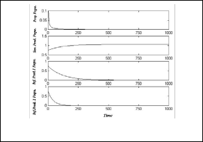
h 1 = 50 , h 2 = 0.01 , h 3 = 0.05 , h 4 = 0.45 , h 5 = 0.06 ,
h 6 = 0.03 , h 7 = 0.45 , e = 0.4 , τ 1 = 0.3 , τ 2 = 0.3
E9
(28)
As shown as in Fig.(9), the system (3) approaches asymptotically to the equilibrium point
E = ( 0 , 8.98, 0.555 , 0.16 ) .
Fig.(6): time series of the trajectories of the system (3)
which shows E6 is a locally asymptotically stable point.
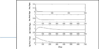
Now to show the stable of second disease free equilibrium
point E7
used the following set of hypothetical parameters
values:
h 1 = 50 , h 2 = 0.8 , h 3 = 0.01 , h 4 = −0.0001 , h 5 = 0.2 ,
h 6 = 0.08 , h 7 = 0.5 , e = 0.5 , τ 1 = 0.4 , τ 2 = 0.8
(26)
As shown as in Fig.(7), the system (3) approaches asymptotically to the stable equilibrium
point E7
= ( 0.013 , 0.344 , 0.046 , 0 ) .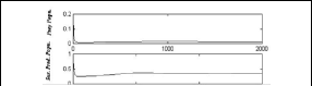
IJSER © 2014 http://www.ijser.
Fig.(9): time series of the trajectories of the system (3)
which shows E9 is a locally asymptotically stable point.
International Journal of Scientific & Engineering Research, Volume 5, Issue 7, July-2014 223
ISSN 2229-5518
Sixth, we have prey-predator model with SIS -disease in predator, investigated the condition (16) for which the
equilibrium point
E7 is stable, and numerically show that
Finally, to understand of dynamical behavior at the
E = ( 0.013 , 0.344 , 0.046 , 0 ) is locally asymptotically stable
coexistence equilibrium point
E10
the following set of
but not globally.
hypothetical parameter values is chosen:
h 1 = 48 , h 2 = 0.88 , h 3 = 0.1 , h 4 = −0.00019 , h 5 = 0.2 ,
(29)
Seventh, we have prey-predator model with SI -disease in predator, investigated the condition (17) for which the
h 6 = 0.08 , h 7 = 0.037 , e = 0.7 , τ 1 = 0.5 , τ 2 = 0.9
equilibrium point
E8 is stable, and numerically show that
As shown as in Fig.(10), the system(3) approaches asymptotically to the stable equilibrium
E8 = ( 0.013 , 0.332 ,0 , 0.342 ) is locally asymptotically stable
but not globally.
point E10
= (0.013 , 0.309 , 0.018 , 0.077 ) .
Eighth, we have epidemic model spread two diseases the population, and investigated in the theorem (10) the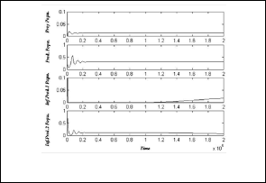
equilibrium point
E9 is stable, and numerically show that
E = ( 0 , 8.98, 0.555 , 0.16 )
is locally asymptotically stable
but not globally.
Finally, we investigated the condition (19) for which the
coexistence equilibrium point
E10
is stable, more than,
numerically prove that
E10
= (0.013 , 0.309 , 0.018 , 0.077 ) is
Fig.(10): time series of the trajectories of the system (3)
which shows E10 is a locally asymptotically stable point.
The stability of model has been studied with linear functional response and numerical response. We propose only one model contain more than one model as following:
First, we investigated that the vanishing equilibrium point
locally asymptotically stable but not globally. In general, use the Lyapunov function to find the stability of the system (3) at each most of its equilibrium points.
[1] Bairagi N., Roy P.K. and Chattopadhyay J., “Role of infection on the stability of a predator–prey system with several response functions– a comparative study”, J. Theo. Biol., 248,10-25, 2007.
[2] Bakare E. A., Adekunle Y. and Nwagwo A., “Mathematical analysis of
the control of the spread of infectious disease in a prey-predator ecosystem”, International Journal of Computer & Organization Trends,
2(1), 27-32, 2012.
[3] Chattopadhyay J. and Arino O., “A predator-prey model with disease
in the prey”, Nonlinear Analysis, 36, 747-766, 1999.
E = (0 , 0 , 0 , 0)
is always unstable, the conditions (10) for
[4] Earn D. J., Dushoff D. J. and Levin S. A., “Ecology and evolution of the
which the axial equilibrium point on the s -axis
E = (0 ,1.059 , 0 , 0 ) is locally asymptotically stable but not
globally, and axial equilibrium point on the p -axis
E = ( 0.02 , 0 , 0 , 0 ) is locally asymptotically stable also it’s
globally.
Second, we have SI - epidemic model with the
flu.”, Trends in Ecology and Evolution, 17, 334-340,2002.
[5] Greenhalgh D. and Haque M., “A predator prey model with disease in the prey species only”, Mathematical Methods in the Applied Sciences, 30,
911-929, 2007.
[6] Haque M. and Greenhalgh D., “When predator avoids infected prey: A model based theoretical studies”, Mathematical Medicine and Biology: a journal to the IMA, 27, 75-94, 2010.
[7] Das K. P., “A Mathematical study of a predator-prey dynamics with
equilibrium point
E3 , and show that
disease in predator”, ISRN Applied Mathematics, 2011, 1-16, 2011.
E = ( 0 , 0.295 , 0 , 2.018 ) is locally asymptotically stable but not globally with conditions (12).
Third, we have SIS - epidemic model with the equilibrium
[8] Haque M. and Venturino E., “An ecoepidemiological model with
disease in predator: the ratio-dependent case”, Mathematical Methods in
the Applied Sciences, 30, 1791-1809, 2007.
[9] Haque M. and Venturino E., “Increase of the prey may decrease the
healthy predator population in presence of disease in the predator”,
point
E4 , and show that, in theorem (5),
HERMIS, 7, 38-59, 2006.
E = (0 , 0.35 , 0.875 , 0)
is locally asymptotically stable but
[10] Haque M., “A predator-prey model with disease in the predator
not globally.
Fourth, we have prey-infected predator by SI model with
species only”, Nonlinear Analysis. RWA, 11(4), 2224-2236, 2010.
[11] Diego J.R. and Lourdes T. S., “Models of infection diseases in spatially
heterogeneous environments”, Bulletin of Mathematical Biology, 63(3),
the equilibrium point
E5 , and show that, in theorem (6),
547–571, 2001.
E = ( 0.014 , 0 , 0 , 0.385 ) is locally asymptotically stable but
not globally.
Fifth, we have prey-predator model with the equilibrium
[12] Liza J.C., Hiroshi A., Noriakiochiai and Makio T., “Biology and predation of the japanese strain of Neosciulus californicus”, Systematic and Applied Acarology, 11, 141–157, 2006.
[13] Das K., Roy S. and Chattopadhyay J., “Effect of disease-selective
point
E6 , and show that, in theorem (7),
predation on prey infected by contact and external sources”,
E = (0.01 , 0.505 , 0 , 0)
is locally asymptotically stable but
BioSystems, 95, 188-199, 2009.
[14] Elisa Elena, Maria Grammauro, Ezio Venturino, “Predator’s
not globally.
alternative food sources do not support ecoepidemics with two strains-diseasedl prey”, Network Biology, 3(1), 29-44, 2013.
IJSER © 2014 http://www.ijser.org
International Journal of Scientific & Engineering Research, Volume 5, Issue 7, July-2014
ISSN 2229-5518
224
[15] Roman F, Rossotto F, Venturino E., "Ecoepidemics with two strains:
diseased predators", WSEAS Tnmsactians on Biology and Biomedicine, 8:
73-85, 2011.
[16] Takeuchi Y., "Global dynamical properties of Lotka-Volterra systems", Singapore,V\brld Scientific, 1996.
[17] Hirsch M. W. and Smale S., "Differential Equation, Dynamical
System, and Linear Algebra", New York, Academic Press,1974.
I£ER lb) 2014 http://WWW.IISer.org