International Journal of Scientific & Engineering Research, Volume 5, Issue 4, April-2014 1087
ISSN 2229-5518
Spectral Analysis of Various Noise Signals
Affecting Mobile Speech Communication
Harish Chander Mahendru, Dr. Ravinder Khanna
—————————— ——————————
PEECH communication is the oldest, cheapest and the most effective mode of communication in the world. It is well known fact that noise is the big enemy of the speech communication. With the advent of mobile phones, although the speech communication is accessible to almost each and every individual, but at the same time it has become more noise prone, due to the fact that it is used in all sorts of noisy environments. Various researchers have addressed this problem in the different ways but none of the speech enhancement algorithm works equally well in all sorts of noise environments and under different signal to noise (SNR) conditions [1]. The research is still on to find out a unique
solution to this problem.
We have taken up this challenge, as part of Ph.D. research,
and have taken up the problem of designing an efficient
speech enhancement algorithm for the mobile communication
which can work in all sorts of noise and SNR conditions. In
this paper we have studied different types of noises which we generally experience during mobile communication, through their spectrum analysis. To make our analysis more realistic, we have recorded the various noise signals in actual noisy environment conditions, described in section–II. We have
————————————————
used Burg’s method to estimate power spectral density for spectral analysis. Different methods of power spectral density analysis are described in section–III. The spectral analysis is done by simulating the actual recorded noise signals using MATLAB signal processing tool (SPtool). The complete process is described in section–IV with the help of graphical representation. Section–V describes the outcomes of the simulation results. The results are concluded in section–VI.
During speech communication through mobile phone, we come across many situations, where there are so many back ground noises, but still we may have to use it. These background noises get mixed with the speech signal and deteriorate its quality and intelligibility. To present realistic analysis, we have recorded different types of noises, ourselves, using Nokia Asha 501 mobile phone, on actual experienced situations. Noise samples, recorded and used for the spectral analysis in this paper, are described below.
Many times we have to use our mobile phone when we are inside the car. We experience car engine noise and the air flow noise (when window is open). We have recorded the car noise in three different situations. (i) When the car engine is on but it is not moving. (ii) When the car is moving at 60
Kmph speed and its windows are closed. (iii) When the car is moving at 60 Kmph speed and its windows are opened. We have recorded these noises in petrol version of Hyundai I-10
IJSER © 2014 http://www.ijser.org
International Journal of Scientific & Engineering Research, Volume 5, Issue 4, April-2014 1088
ISSN 2229-5518
Kappa engine model of the car, while driving on state highway from Yamuna Nagar to Kurukshetra.
These are the noises that we generally experience while at home or office, especially during summer when ceiling fan or exhaust fan is on in the room. We have recorded two different situations of the room noise. (i) Exhaust fan noise, recorded at about 2 feet away from the exhaust fan. (ii) Ceiling fan noise, recorded at about 7 feet away from the ceiling fan.
When we are at railway platform, we experience background noises of train arrival/departure and in between regular train announcements. When we are traveling inside the train, we experience background noises in the form of talks of fellow passengers and the sounds produced due to the train movement. Here we have recorded sounds in four different situations. (i) Railway platform train announcement noise. (ii) Railway platform train arrival noise. (iii) Inside train compartment moving at slow speed. (iv) Inside train compartment moving at fast speed.
The street noise has been recorded while traveling inside a three wheeler auto on busy city road.
This type of sound is produced when so many people talk together. Sound of such a situation is recorded inside a college classroom when students are talking to each other in the absence of a teacher.
All the speech and noise signals are random in nature. They are constituted of multiple wide ranges of frequencies. Distribution of power contents of different frequency constituents in the signal is known as power spectral density. Frequency wise analysis of the time domain random signal process is known as spectral analysis [2], [3]. Let the noise signal is represented as x(t), in continuous time domain. The Fourier transform of the signal x(t) is given by
![]() (1) The signal energy is then given by Parseval’s relation as,
(1) The signal energy is then given by Parseval’s relation as,
Let Sxx(f) represents energy spectral density of the signal at specific frequency f then it is given by
![]() (3) Where F{Rxx(τ)} is the Fourier transform of the
(3) Where F{Rxx(τ)} is the Fourier transform of the
autocorrelation function Rxx(τ) of the signal x(t). Plot of
│X(f)│2 versus frequency f is called power spectrum.
Let x(n) represents the sampled version of the signal x(t),
sampled at sampling frequency fs. Then for a time limited signal having N point sequence, the estimate of power spectral density Pxx(f), known as periodogram, is given by Weiner–Khinchine theorem,![]() (4) Where rxx (k) is the autocorrelation function of the sequence.
(4) Where rxx (k) is the autocorrelation function of the sequence.
In the non parametric methods, PSD is estimated directly from the signal and no assumption is made about how the data is generated. Periodogram, Bartlett, Welch, Blackman & Turkey, and Multi taper are few non parametric methods of PSD estimation. These methods are simple in computation but they require long data sequences and have leakage effects because of windowing [4], [5].
These are modeling based methods in which signal whose PSD is to be estimated is assumed to be output of a linear system driven by white noise. In these methods firstly the parameters (coefficients) of the linear system that hypothetically generates the signal are estimated. Based on these parameters, then, the PSD of the given signal is obtained. Yule Walker autoregressive (AR), Burg AR, Covariance and Modified covariance methods are few examples of parametric methods [4], [5].
These methods generate frequency component estimates for a signal based on an Eigen analysis or Eigen decomposition of the correlation matrix. These methods are also known as high resolution or super resolution methods and are useful in the detection of sinusoids buried in noise, especially when the signal to noise ratio is low. Multiple signal classification (MUSIC) and the eigenvector (EV) methods are few examples of subspace methods.
![]() (2)
(2)
IJSER © 2014 http://www.ijser.org
International Journal of Scientific & Engineering Research, Volume 5, Issue 4, April-2014 1089
ISSN 2229-5518
In this paper we have used Burg’s method for power spectral analysis of noise signals because it is more stable, provides high frequency resolution for short data records and is computationally efficient than other methods. It gives smoother results over whole frequency range of the spectrum. It is based on minimizing the forward and backward prediction errors while satisfying the Levinson-Durbin recursion. It avoids calculating the autocorrelation function, and instead estimates the reflection coefficients directly.
For a sampled sequence x(n), having N-1 samples,
the Burg’s PSD is given as,
![]() (5) Where Êp is the total squared error estimate of the auto
(5) Where Êp is the total squared error estimate of the auto
recursive (AR) process of order p. In our present analysis, we
have used order p = 10 and N(fft) =1024.
We have recorded the sounds in different noise environments using Nokia Asha-501 mobile phone. It records the sound in
.amr format. These files have been converted to .wav format, the acceptable format for sound signals in MATLAB, using online file converter software available at [6]. These files are then imported into the workspace of MATLAB [7]. The noise signal data is stored in the workspace in the form of a column vector that represents the magnitudes of the signal at different sample points. Since frequency bandwidth of the speech signal is contained within 4 KHz, all the noise signals are sampled at 8 KHz (the Nyquist sampling rate). Let t is the duration of a particular noise recording then total samples, N, contained in the column vector is given by,
N = t*8000 + 1 (6) But to keep constant sample values for all the noise signals
we have sliced them for 5 second duration only, from 10th
second of recording to 15th second of recording, by using
MATLAB command given by,
XX_5s = XX(80000:120000) (7) Where XX is the respective variable name of the original
recorded noise signal column vector and XX_5s is variable
name assigned to the sliced column vector.
Fig. 1, 2 and 3 show the 5 second sliced sampled signals of car noises, recorded in three different conditions as described in section 2.1.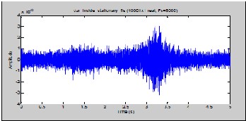
Fig. 1 Sampled signal of car cabin when engine is on but it is not moving.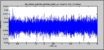
Fig. 2 Sampled signal of car cabin when car is moving at 60
Kmph, windows closed.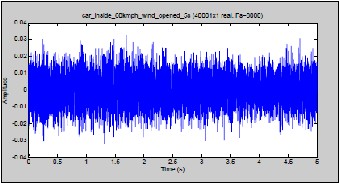
Fig. 3 Sampled signal of car cabin when car is moving at 60
Kmph, windows opened.
Fig. 4, 5 and 6 show the Burg’s power spectral density distribution of the above three types of car noises, obtained using MATLAB’s signal processing tool box.
IJSER © 2014 http://www.ijser.org
International Journal of Scientific & Engineering Research, Volume 5, Issue 4, April-2014 1090
ISSN 2229-5518
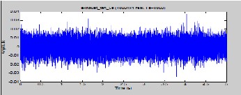
Fig. 4 Burg’s PSD of car cabin when engine is on but it is not moving.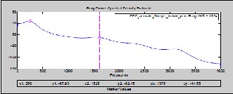
Fig. 5 Burg’s PSD of car cabin when car is moving at 60
Kmph, windows closed.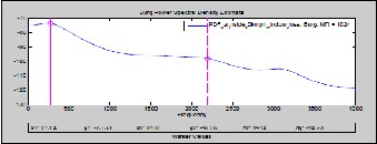
Fig. 6 Burg’s PSD of car cabin when car is moving at 60
Kmph, windows opened.
Figures 7 and 8 show the 5second sliced sampled signals of ceiling fan and exhaust fan noises, respectively, that we generally experience in a room.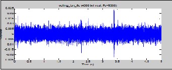
Fig. 7 Sampled signal of ceiling fan noise.
Fig. 8 Sampled signal of exhaust fan noise.
Figures 9 and 10 show the Burg’s power spectral density distribution of the above two types of room noises, obtained using MATLAB’s signal processing tool box.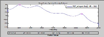
Fig. 9 Burg’s PSD of ceiling fan noise.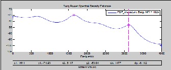
Fig. 10 Burg’s PSD of exhaust fan noise.
Figures 11, 12, 13 and 14 show the 5second sliced sampled signals of railway platform and train noises as described in section 2.3.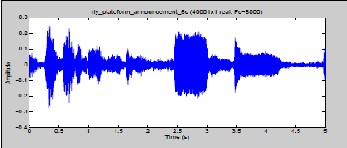
Fig. 11 Sampled signal of railway platform train announcement noise.
IJSER © 2014 http://www.ijser.org
International Journal of Scientific & Engineering Research, Volume 5, Issue 4, April-2014 1091
ISSN 2229-5518
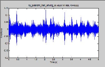
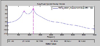
Fig. 15 Burg’s PSD of railway platform during train announcement.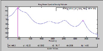
Fig. 12 Sampled signal of railway platform noise when train is arriving on the platform.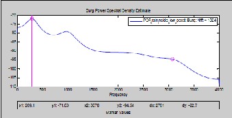
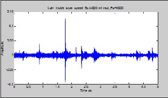 Fig. 16 Burg’s PSD of railway platform during train arrival.
Fig. 13 Sampled signal of train cabin when it is moving at slow speed.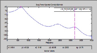
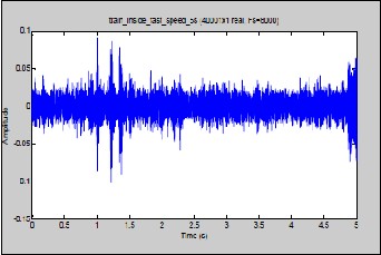 Fig. 17 Burg’s PSD of train cabin, moving at slow speed.
Fig. 14 Sampled signal of train cabin when it is moving at fast speed.
Figures 15, 16, 17 and 18 show the Burg’s power spectral density distributions of the above four types of train noises, obtained using MATLAB’s signal processing tool box.
Fig. 18 Burg’s PSD of train cabin, moving at fast speed.
IJSER © 2014 http://www.ijser.org
International Journal of Scientific & Engineering Research, Volume 5, Issue 4, April-2014 1092
ISSN 2229-5518
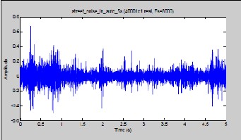
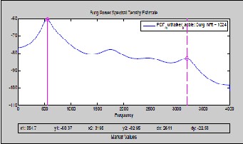
Figure 19 shows the 5second sliced sampled signal of street noise recorded while traveling in a three wheeler auto on a busy road and figure 20 shows its PSD estimation.
Fig. 22 Burg’s PDF of multi talker babble noise.
Fig. 19 Sampled signal of street noise of a busy city road.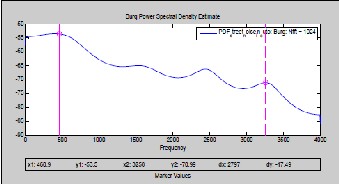
Fig. 20 Burg’s PSD of street noise of a busy city road.
Figure 21 shows the 5second sliced sampled signal of multi talker babble noise recorded as described in section 2.5 and figure 22 shows its PSD estimation.
From the power density distribution of various noise signals, following outcomes are summarized.
Power density (PD) increases from -95 dB at 0 Hz to -92 dB at
211 Hz (Max PD). It decreases thereafter until -117 dB at 2281
Hz and starts rising again thereafter until -105 dB at 3100 Hz. From this point it starts decreasing again with minimum -125 dB at 4 KHz.
Its PD increases from -70 dB at 0 Hz to -68 dB at 234 Hz (Max PD). Further it decreases continuously with minimum -105 dB at 4 KHz. Small crests can be seen at frequency points 1596
Hz, 2359 Hz and 3132 Hz.
Its PD increases from -75 dB at 0 Hz to -73 dB at 249 Hz (Max PD). Further it decreases continuously with minimum -120 dB at 4 KHz. Small crests can be seen at frequency points 2174
Hz and 3085 Hz.
Its PD increases from -87 dB at 0 Hz to -80 dB at 486 Hz (Max PD). Further decreases continuously with minimum -107 dB at 4 KHz. Noticeable crests can be seen at frequency points
1288 Hz (-81dB) and 3252 Hz (-92 dB). There is very small crest at frequency point 2366 Hz.
Fig. 21 Sampled signal of multi talker babble noise.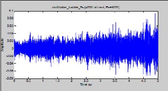
Its PD decreases from -75 dB at 0 Hz to -81 dB at 1192 Hz. It increases thereafter until -75 dB (Max PD) at 1666 Hz. It decreases continuously from this point with minimum -100 dB at 4 KHz. One noticeable crest is seen at frequency point
3115 Hz (PD -83 dB).
IJSER © 2014 http://www.ijser.org
International Journal of Scientific & Engineering Research, Volume 5, Issue 4, April-2014 1093
ISSN 2229-5518
Spectral density distribution of this type of noise is slightly different from above types of noises. Its PD first increases from -82 dB at 0 Hz to -52 dB at 748 Hz. Having deep valley at
930 Hz (-61 dB), it increases up to maximum PD of -48 dB at
1172 Hz and thereafter decreases continuously from this point
with minimum -98 dB at 4 KHz.
Its PD increases from -71 dB at 0 Hz to -62 dB (Max PD) at 443
Hz. It decreases thereafter until -80 dB at 1437 Hz. From this
frequency point to 3360 Hz it has almost constant PD with
small crests at frequency points 1831 Hz, 2530 Hz and a deep
valley at 2978 Hz (-83 dB). From frequency point 3360 Hz, it keeps on decreasing with minimum PD of -91 dB at 4 KHz.
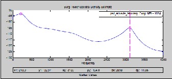
Its PD increases from -79 dB at 0 Hz to -71 dB (Max PD) at 297
Hz. It decreases thereafter until -109 dB 4 KHz. In between it has a noticeable crest at 1 KHz (PD -79 dB) may be the sound of train whistle.
Its PD increases from -74 dB at 0 Hz to -65 dB (Max PD) at 664
Hz. It decreases thereafter until -104 dB 4 KHz. In between it
has two noticeable crests at 2383 Hz (PD -86 dB) and at 3203
Hz (PD -90 dB).
Its PD decreases continuously from -57 dB at 0 Hz to -86 dB at
4 KHz. In between it has few crests at 453 Hz (PD -53 dB -
Max), at 1586 Hz (PD -65 dB), at 2445 Hz (PD -66 dB), and at
3273 Hz (PD -71 dB).
Its PD first increases from -79 dB at 0 Hz to -60 dB (Max PD)
at 555 Hz and then decreases continuously up to -101 dB at 4
KHz, having crests, in between, mainly at 3188 Hz (PD -83
dB) and at 1750 Hz (PD -78 dB).
derived in this paper can be useful in noise modeling while designing speech enhancement algorithms for mobile communication. As further study to this research work, comparative spectrum analysis of the above noise signals with standard random processes such as Gaussian, Laplacian, Gamma etc. can be made for efficient noise modeling.
[1] Yi Hu, and Philipos C. Loizou, “Subjective comparison and evaluation of speech enhancement algorithms”, Elsevier, Speech Communication, 49, 2007, 588-
601.
[2] Proakis, J.G., and D.G. Manolakis, Digital signal processing: principles, algorithms, and applications, Englewood Cliffs, NJ: Prentice Hall, 1996.
[3] Hayes, M.H., Statistical digital signal processing and modeling, New York: John
Wiley & Sons, 1996.
[4] Kay, S.M., Modern Spectral Estimation, Englewood Cliffs, NJ: Prentice Hall,
1988.
[5] Marple, S.L., Digital Spectral Analysis, Englewood Cliffs, NJ: Prentice Hall, 1987.
[6] www.convertfiles.com.
[7] Signal Processing Tool Box, User’s guide, version 4.2, Math Works
Incorporation..
An effort has been made in this paper to analyse spectral properties of different types of noises those are generally experienced in different noisy environments while using mobile phone. From the outcomes of the results, stated above, we can infer that all types of noises have wide bandwidth with power density spread from 0 Hz to 4 KHz. However most of the energy is distributed over the lower frequency band i.e. up to 1500 Hz. Some noticeable energy peaks are also observed, in few noise cases, over the higher frequency band i.e. between 1.5 KHz to 4 KHz. Spectrum analysis
IJSER © 2014 http://www.ijser.org