International Journal of Scientific & Engineering Research, Volume 5, Issue 4, April-2014 1130
ISSN 2229-5518
Solving the Problem of Mismatched Loads in High Voltage Networks Applying Power Circle Diagram Technique
Assistant Professor Mohammed Sabri A. Raheem *
ABSTRACT: This paper deals mainly with the problem of mismatched loads with the power networks and to discuss the solution for this problem by the insertion of reactive power at the receiving end terminal. The process is basically calculated applying the Receiving End Power Diagram Analysis method , which gives an easier & faster calculating process ,also a computer program is constructed to perform the calculation and selection process. The network condition ,taken as a case study example load, can be changed and the calculation process is performed ,hence the results will be discussed for each system parameters
KEY W ORDS: Power Factor Improvement, Reactive Power Injection , Power Circle Diagram , T.L. General Parameters .
1- INTRODUCTION
Delivering electric energy to loads, especially at peak loads periods, forms a challenge task to the electric utility control [1]
. The problem arises when there is a mismatching in the
parameters between sending, receiving end network terminals, for which a T.L. forms the electric media for the power transmission [2] .
The power circle diagram technique gives simple solution
methodology that relates send. ,T.L. & receiving end parts of the network, hence presenting a locus diagram that assists the utility engineer in correcting the problems arises during The network operating conditions , especially on different load fluctuations [3] .
The task here seems to be similar to the criteria of power factor correction, by adding reactive power to the network, but here the aim is to locate the receiving end load point on the locus of the power circle diagram & solve the mismatching problem rather than adding reactive power to improve the p.f. [4,5].

* Assist. Prof. Mohammed Sabri is working at the College of Electrical & Electronic Techniques , Foundation Of Technical Education – Baghdad – Iraq .
E Mail. mohsab2008@gmail.com
Moreover for the network shown in figure (1A) ,& of the voltage phasor of figure (1B), the electric power system voltage equations are :[6]
𝑽𝒔 = 𝑨 𝑽𝒓 + 𝑩 𝑰𝒓 ------ ( 1 )
Converting the system of eq. (1) above to a power equation
yields to the form of equation (2),below

𝑷𝒍𝒐𝒂𝒅 = (𝑽𝒔∗𝑽𝒓) 𝒄𝒐𝒔(𝜷 − б) − �𝑨 𝑽𝒓𝟐 /𝑩� 𝒄𝒐𝒔(𝜷 − 𝜶) ----------
𝑩
- ( 2 )
From this equation it is possible to draw the power circle diagram for the case of network conditions of equations (1) & (2) and as shown in figure (2) below .
From what is shown in figure (2) & equation (2) above , it can
be noted that the operating torque angle (δ) is calculated from equation (3) below & to be compared with that found from figure (2) above :

𝒄𝒐𝒔−𝟏�𝑷𝒍𝒐𝒂𝒅 + 𝑨𝑽𝒓𝟐 𝒄𝒐𝒔(𝜷−𝜶)�
𝜹 = 𝜷 − -------- ( 3 )
𝑽𝒔𝑽𝒓/𝑩
2- POWER CIRCLE DIAGRAM TECHNIQUE
The power circle diagram technique is initialized taking the case of the network shown in fig. (1A) ,and for a load condition of a lagging p.f. load.
The T.L. is to be represented by its general matrix
(A,B,C,D) parameters for which the voltage phasor diagram is shown in fig(1B).
IJSER © 2014 http://www.ijser.org
International Journal of Scientific & Engineering Research, Volume 5, Issue 4, April-2014 1131
ISSN 2229-5518
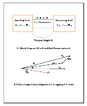
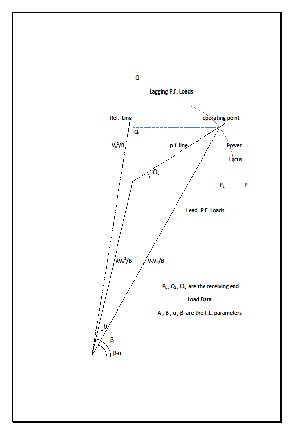
Figure (1) Power Network System
A, B, α, & β are the T.L. parameters.
It is noted also from above that if the load point does not locate on the power circle diagram locus , there will be a need to insert a reactive power at the receiving end (inductive or capacitive) to force the load point to be moved vertically, hence located on the locus , as in Fig.(3) , with an additional reactive power ( Qadd. )
as in equation (4) below :
𝑸𝒂𝒅𝒅. = 𝑸𝑹𝒆𝒄. − 𝑸𝑳𝒐𝒄𝒖𝒔 ------------- ( 4 )
Where :
Qadd | , | the additional reactive power . |
QRec. | , | = Received = = . |
QLocus | , | the locus point reactive power . |
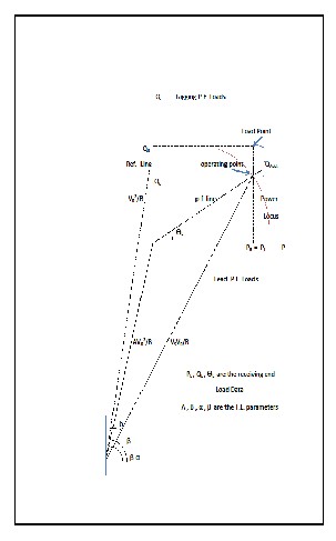
Figure (3) Detailed Power Circle Diagram
Where :
(2) Basic Power Circle Diagram
Figure
3- NET WORK SYSTEM CASE STUDY
For a case study to be considered as a power system
VS , VR are the Sending & Receiving End Voltages
respectively
condition , the power network parameters are as below :
IJSER © 2014 http://www.ijser.org
International Journal of Scientific & Engineering Research, Volume 5, Issue 4, April-2014 1132
ISSN 2229-5518
VS = 440 Kv , VR = 400 Kv ,
A = 0.9 ∟5o , B = 10 ∟80o Ω
& for a constant lagging p.f. load of 0.866 .
For the network data above two solution methods had
a) For a comparative purposes the same torque angles (б) is taken as an input data, more over & for the network data given (б) can be calculated applying equation (5) ,
−𝟏
been carried out & the solutions are compared, the TWO
solution procedures are :

𝜹 = 𝟖𝟎 − 𝒄𝒐𝒔
(𝑷𝒍𝒐𝒂𝒅 + 𝟏𝟓.𝟒 𝒄𝒐𝒔 𝟕𝟓)
𝟏𝟕.𝟔
------- ( 5 )
3-1 : POWER CIRCLE DIAGRAM DRAWING METHDOLOGY
According to figure (2) , a load active power of ( 1 GW – 10
GW ) at a constant lagging p.f. of (0.866) , ,leads to the data obtained in Table (1) , and the condition of the operating point shows the need for adding reactive power according to the power locus
& the power factor line alignments :
b) From equation (2) above , the locus active power is calculated (PR ) , then the reactive power is calculated for a
0.866 lagging p.f. load.
c) The calculated reactive power is compared with that of power locus diagram ( QLocus ).
d) If the TWO reactive powers does not coincide , there will be
a need for reactive power injection , of values of ( QLocus – Q
R ) .
The above algorithm results are listed in Table (2) below & the differences between the TWO solution methodologies can be noticed. The majority of the differences of results comes from the choice of the
drawing scale & of course the accuracy in the eq.
calculations methodology.
10 10
10 10
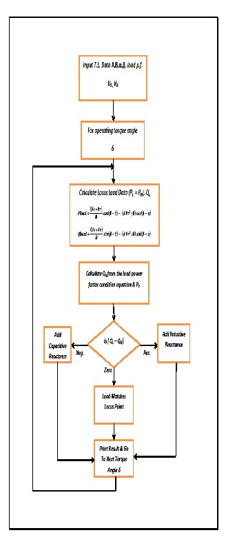
3-3 : THE COMPUTER PROGRAM FLOW CHART
The flow chart of the computer program is shown in figure (4) below. Assuming the followings ,just for calculations & case study comparative purposes :
a) The power factor , load condition & the active power values .
b) The torque angles (б) is as found in the power circle diagram drawing method & hence taken to be the values of the system operating torque angles .
What is noted from this flow chart , the followings :
1 ) The main statement deciding the type of additional reactive power is as in equation ( 6 ):
Table (1) Power Circle Diagram Solution Data
3-2 : COMPUTER PROGRAM SOLUTION METHDOLOGY
As an alternative & more accurate solution method is carried out , a computer program is constructed to
calculate the necessary network parameters as given in the
algorithm below :
𝑸 𝑨𝒅𝒅𝒊𝒕𝒊𝒐𝒏𝒂𝒍 = 𝑸 𝑹𝒆𝒄.𝑬𝒏𝒅 − 𝑸 𝑳𝒐𝒄𝒖𝒔 ------- ( 6 )
Where the conditions are :
a- Adding Inductive Reactive Power for the case of
QAdditional Negative .
b- Adding Capacitive Reactive Power For the case of QAdditional Positive .
c- The Rec. End Load point Coincide with the Power
Locus Point ( QAdditional =Zero ) .
IJSER © 2014
http://www.ijser.org
International Journal of Scientific & Engineering Research, Volume 5, Issue 4, April-2014 1133
ISSN 2229-5518
2) The construction of the computer program presents
a more accurate methodology for choosing the proper additional reactive power to match the load & the T.L.
system.
10 10
10 10
Table (
2 )
Progra m Method ology Solution Data
Figure (4) Program Flow Chart
IJSER © 2014 http://www.ijser.org
International Journal of Scientific & Engineering Research, Volume 5, Issue 4, April-2014 1134
ISSN 2229-5518
4 – CONCLUSIONS
Two comparable methods had been presented to solve the problem of mismatching of the electric load with the network parameters .
The solution method based on the construction of the power circle diagram .
The two solution approaches are mainly :
1 ) The drawing of the power circle diagram & find the necessary data from the drawing where the effect of the drawing scale & angles measurement affects directly the accuracy of the data obtained , but gives a fast & easy solution method ( data of Table ( 1 ) ).
2 ) The equations ( that are necessary to construct
the circle diagram ) are used , with necessary assumptions , to construct the computer program calculation method giving a more accurate way to find the solution results , data of Table ( 2 ) , .
What forms the dominant factor for both methods is the
operating torque angle , that is found from the drawing method & forms the basic operating torque angles for the computer program method. This is set just to show a basic comparison & solution calculation methodology.
The solution approach presented in the paper had been
performed for two-port network ,namely, sending & receiving end terminals . For other networks the approach should be little modified to fit the other networks
formulations.
1 – J.D.Glover & M.S.Sarma , “ Power System Analysis & Design “ ,The Wadsworth Group ,Thomson Learning , Inc.
, Third Edition, 2002 .
2 – B.R.Gupta ,“Power System Analysis & Design
“,S.Chand & Company Ltd ., Fifth Revised Edition ,2008 .
3- Chard F. de la C., "Transmission-line estimations by combined power circle diagrams", Proceedings of the IEE
- Part IV : Institution Monographs , vol.101, no.7,
pp.204,208, August 1954 .
4 – M.S. A.Raheem , “Optimal Reactive Power Insertion
& Allocation To The Iraqi Super Grid 400 Kv Network Applying Genetic Algorithm Technology “ , International Journal of & Scientific Engineering Research, IJSER , Vol. 4 , Issue 12, December-2013 .
5 - A. M. Sharaf and S. T. Ibrahim, “Optimal Capacitor Placement in Distribution networks", Electric Power System Research, no. 37, pp. 181–187
, 1996.
6 – M. S .A .Raheem , “ Transmission & Distribution Lecture Notes “ , Electric Power Techniques Dept . , College Of Electric & Electronic Techniques , Baghdad – Iraq , 2013 .
5- REFRENCES
IJSER © 2014 http://www.ijser.org