InternationalJournalofScientific&EngineeringResearchVolume 2, Issue 4, April-2011 1

ISSN 2229-5518

SLANT TRANSFORMATION AS A TOOL FOR PRE-PROCESSING IN IMAGE PROCESSING Nagaraj B Patil, V M Viswanatha , Dr. Sanjay Pande M B

Abstract—The Slantlet Transform (SLT) is a recently developed multiresolution technique especially well-suited for piecewise linear data. The Slantlet transform is an orthogonal Discrete Wavelet Transform (DWT) with 2 zero moments and with improved time localization. It also retains the basic characteristics of the usual filterbank such as octave band characteristic and a scale dila- tion factor of two. However, the Slantlet transform is based on the principle of designing different filters for different scales unlike iterated filterbank approaches for the DWT. In the proposed system, Slantlet transform is implemented and used in Compression

and Denoising of various input images. The performance of Slantlet Transform in terms of Compression Ratio (CR), Reconstruc- tion Ratio (RR) and Peak-Signal-to-Noise-Ratio (PSNR) present in the reconstructed images is evaluated. Simulation results are discussed to demonstrate the effectiveness of the proposed method.

Index Terms—Discrete Wavelet transform, Compression ratio, Data Compresion, Peak-signal-to-ratio(PNSR), Coding Inter Pixel, Slantlet Coefficients, Choppy Images.

—————————— • ——————————

1 INTRODUCTION

or many decades, scientists wanted more appropriate functions than the sines and cosines, which comprise
the basis of Fourier analysis, to approximate choppy im- ages. By their definition, these functions are non-local (and stretch out to infinity). Therefore they do a very poor job in approximating sharp spikes. Wavelets are functions that satisfy certain mathematical requirements and are used in representing data or other functions.
This makes wavelets interesting and useful. But with wavelet analysis, approximating functions can be used that are contained neatly in finite domains. Wavelets are well suited for approximating data with sharp discon- tinuities [1].
The Discrete Wavelet transform (DWT) is usually
carried out by filterbank iteration, but for a fixed number

————————————————

• Nagaraj B Patil is currently pursuing. Ph.Dfrom Singhania University Rajastan. At present he is working as Asst. Prof. and HOD Dept. of CSE, Govt. Engg. College Raichur. E-mail: nagarajbpatil@yahoo.co.in

• V M Viswanatha is currently pursuing Ph.D from Singhania University,

Rajastan. At present he is working as a Asst. Professor , E&CE Dept. at

SLN College of Engg. Raichur E-mail: vmviswanatha@gmail.com

• Dr. Sanjaya Pandey , At present is working as a Prof. and HOD Dept. of

CSE at VVIT, Mysore. E-mail: rakroop99@gmail.com
of zero moments it does not yield a discrete time basis that is optimal with respect to time localization. The Slantlet transform is an orthogonal DWT with 2 zero moments and with improved time localization. The Slant- let transform has been developed by employing the lengths of the discrete time basis function and their mo- ments as the vehicle in such a way that both time- localization and smoothness properties are achieved. Us- ing Slantlet transform it is possible to design filters of shorter length while satisfying orthogonality and zero moments condition. The basis function retains the octave- band characteristic. Thus Slantlet transform has been used as a tool in devising an efficient method for com- pression and denoising of various images.

2. Literature survey

G.K. Kharate, A.A. Ghatol, et.al [2], proposed an algorithm based on decomposition of images using Dau- bechies wavelet basis. Compression of data is based on reduction of redundancy and irrelevancy. They have pro- posed an adaptive threshold for quantization, which is based on the type of wavelet, level of decomposition and
nature of data.

International Journal of Scientific & Engineering Research Volume 2, Issue 4, April-2011 2

ISSN 2229-5518

Sos S. Agaian, Khaled Tourshan, et.al [3] propos- es a novel approach for the parameterization of the slant- let transform with the classical slantlet and the Haar transforms are special cases of it is presented. The slantlet transform matrices are constructed first and then the fil- terbank is derived from them. The parametric slantlet transform performance in image and signal denoising is discussed.
Panda. G, Dash. P K, et.al [4] proposes a novel approach for power quality data compression using the slantlet is presented and its performance in terms of com- pression ratio (CR), percentage of energy retained and mean square error present in the reconstructed image is assessed.
Lakhwinder Kaur, Savita Gupta, et.al [5] pro- posed an adaptive threshold estimation method for image denoising in the wavelet domain based on the genera- lized Guassian distribution (GGD) modeling of subband coefficients.
Lei Zhang; Bao, P; Xiaolin Wu [8] proposed a wavelet-based multiscale linear minimum mean square- error estimation (LMMSE) scheme for image denoising is proposed, and the determination of the optimal wavelet basis with respect to the proposed scheme is discussed. The overcomplete wavelet expansion (OWE), which is more effective than the orthogonal wavelet transform (OWT) in noise reduction, is used.

3.The Slantlet Transform

The Slantlet filterbank is an orthogonal filter bank for the discrete wavelet transform, where the filters are of shorter support than those of the iterated D2 filter- bank tree. This filterbank retains the desirable characteris- tics of the usual DWT filterbank.

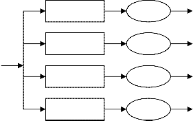
The Slantlet filter bank shown in Fig 3.1. is generalized as follows. The l-scale filter bank has 2l channels. The low-

pass filter is to be called hl(n). The filter adjacent to the

lowpass channel is to be called fl (n). Both hl(n) & fl(n) are to be followed by down sampling by 2l. The remaining 2l

- 2 channels are filtered by gi(n) & its shifted time-reverse for i =1,…., l-1. Each is to be followed by down sampling by 2i+1. x(n) Slantlet filter Coefficients

H2(Z) 4

F2(Z) 4

G1(Z) 4

Z-3 G1(1/Z) 4

Fig 3.1. Slantlet filterbank

In the Slantlet filterbank, each filter gi(n) does not appear together with its time reverse. While hi(n) does not
appear with its time reverse, it always appears
paired with the filter fi(n). In addition, note that the l-scale and (l + 1) scale filterbanks have in common the filters gi(n) for i=1,…., l-1 and their time-reversed versions.
The Slantlet filterbank analyzes scale i with the filter gi(n) of length 2i+1. The characteristics of the Slantlet filterbank:
1.Each filterbank is orthogonal. The filters in the synthe- sis filter bank are obtained by time reversal of the analysis filter.
2.The scale-dilation factor is 2 for each filterbank.
3.Each filterbank provides a multiresolution decomposi- tion.
4.The time localization is improved with a degradation of frequency selectivity.
5.The Slantlet filters are piecewise linear.

4.Compression

The term data compression refers to the process of reducing the amount of data required to represent a

International Journal of Scientific & Engineering Research Volume 2, Issue 4, April-2011 3

ISSN 2229-5518

given quantity of information. It is useful both for trans- mission and storage of information[7].

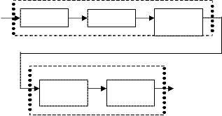
The encoder of the Fig 4.1 is responsible for re- ducing the coding interpixel and/or psychovisual redun- dancy of the input data. In the first stage of the encoding process the mapper transforms the input data into a for- mat designed to reduce the interpixel redundancies.

output data is generated. Error can be defined between f and f1

e = f1- f ………..4.1

The decoder contains only two components: a symbol decoder and an inverse mapper. The percentage of reconstruction ratio can be defined as

Vector norm of the retained SLT Coefficients after threshold

X100

Vector norm of the original SLT coefficients

Mapper

Quantizer

Encoder

Symbol

coder

Compression of data without degradation of data

Symbol decoder

Decoder

Inverse

Mapper

Compressed data

quality is possible because the data contains a high degree of redundancy. The higher the redundancy the higher the achievable compression. The data compression methods can be broadly classified into

1. Lossless compression method

Fig4.1.General Block diagram for compression

The second stage, or quantizer block, reduces the accuracy of the mappers output in accordance with a predifined fidelity criterion- attempting to eliminate only psychovisually redundant data. This operation is irrevers- ible and must be omitted when error-free compression is desired. In the third and final stage of process, a symbol coder creates a code (that reduces coding redundancy) for the quantizer output and maps the output in accordance with the code.

If n1 and n2 denotes the number of informations carrying units in the original and encoded data respec- tively, the compression that is achieved can be quantified numerically via the compression ratio

CR = n1/n2

To view and/or use a compressed (i.e., encoded)

data, it must be fed into a decoder, where a reconstructed

2. Lossy compression method.

5.DENOISING

The de-noising objective is to suppress the noise part of the signal s and to recover f while retaining as much as possible the important signal features.

The noisy signal is basically of the form

s(n) = f(n) + cre(n), where e(n) is the gaussian white noise

N(0,1) and time n is equally spaced.

In the recent years there has been a fair amount of research on wavelet threshold and threshold selection for image de-noising, because wavelet provides an ap- propriate basis for separating noisy signal from the data signal. Threshold is a simple non-linear technique, which operates on one wavelet coefficient at a time. Replacing the small noisy coefficients by zero and inverse wavelet transform on the result may lead to reconstruction with the essential signal characteristics and with less noise. The

International Journal of Scientific & Engineering Research Volume 2, Issue 4, April-2011 4

ISSN 2229-5518

Peak-Signal-To-Noise-Ratio(PSNR) for any given data can be given as, PSNR=20*log10(1256/ (original data-de- noised data)).

6.Design Procedure

6.1.Algorithm for signal compression

The design procedure for signal compression contains three steps:

1. Decomposition

The Slantlet transform is used for decomposition and applied to each row and then again applied to the resulting information in each column. The steps used for decomposition

1.Find out whether the input signal is power of 2.

1.2. Separate the odd and even moment vectors along the length of the input signal.

1.3. Since the filters are piecewise linear, each filter can be represented as the sum of a DC and a linear term.

1.4. The DC and linear moments at scale i can be com- puted from the DC and linear moments at the next finer scale (i-1).

The image obtained after 2-D Slantlet transform can be shown as

Figure 5.3. Decomposed image after 2-D Slantlet Trans- form

2. Threshold the coefficients

If a pixel in the image has intensity less than the threshold value, the corresponding pixel in the resultant image is set to white. Otherwise, if the pixel is greater
than or equal to the threshold intensity, the resulting pix-
el is set to black. Soft threshold is used for image com- pression.

3.Reconstruction

Compute wavelet reconstruction based on the modified coefficients. This step uses the inverse Slantlet transform to perform the wavelet reconstruction.
3.1. Find out whether the signal is of finite duration
(power of 2).
3.2. Initialize the moment vectors.
J.0 = 1:N/2
J.1 = J.0
3.3. Using DC and linear Slantlet coefficients, compute
J.0(n;l) and J.1(n;l)
m = 2^l;
J.0(n;l)=s(1)/Y(m)*s(2)*Y(3*(m-1)/(m*(m+ 1)));
J.1(n;l) = s(2) * (-2 * Y(3/(m*(m^2 - 1)))
3.4. Then compute J.0(n;i) and J.1(n;i) for decreasing val- ues of i by updating J.0 and J.1 using Slantlet coefficients.

6.2. Algorithm for signal De-noising

Input image is added with noise. For this noisy image, apply Slantlet transform. Steps 1 and 3 of the sec- tion 6.1 remains unchanged. But in the step 2, soft thre- shold is applied for de-noising. Soft threshold is an exten- sion of hard threshold, first setting to zero the elements whose absolute values are lower than the threshold, and then shrinking the nonzero coefficients towards 0. The output of the step3 in section 6.1 is the de-noised version of the original input image.

7. Results and Analysis

Computer simulation study on Compression and De-nosing were carried out on some standard images to the Matlab programs of the Slantlet transform. Some 2D inputs include images of a cameraman, MRI and Testpart. Implementation is carried out using Matlab.

7.1. Simulation Results of Compression

International Journal of Scientific & Engineering Research Volume 2, Issue 4, April-2011 5

ISSN 2229-5518

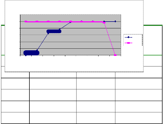
The Compression Ratio (CR) and Reconstruction

Ratio (RR) for different input images are tabulated as

shown in the table 6.1 and table 6.2. The graphs are plot- ted against various threshold values and the ratios.

Thr value	Cameraman	MRI	Testpart
Thr value	% CR	% RR	% CR	% RR	% CR	% RR
0	0	100	0	100	0	100
0. 5	14.73	100	52.95	99.99	11.68	100
5.0	64.68	99.99	70.10	99.97	54.25	99.99
10.0	76.02	99.99	79.92	99.87	69.92	99.99
100	98.02	99.80	98.86	96.66	95.97	99.69
500	99.81	99.24	99.81	89.28	99.60	98.07
5000	99.97	96.22	99.99	18.79	99.97	94.74

Table 7.1. Percentage of Compression Ratio(CR) and

Reconstruction Ratio(RR) for different Images

Figure 7.1. Graph for Cameraman

7.2. Simulation results of de-noising

For the various threshold values, the percentage of signal to noise ratio for different images are tabulated as shown in the table 6.3 and 6.4. The graphs are plotted against various threshold values and the PSNR.

120

100

%Cr

0 0. 5 5 10 100 500 1000 5000 50000

Threshold

% RR art)

Table 7.2. Percentage of Signal to noise ratio (PSNR) for dif-

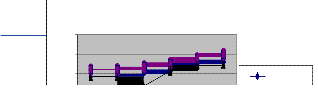
ferent Images

Cameraman

International Journal of Scientific & Engineering Research Volume 2, Issue 4, April-2011 6

ISSN 2229-5518

Figure 7.2. Graph between Threshold and PSNR for different

Images.

8. Snapshots

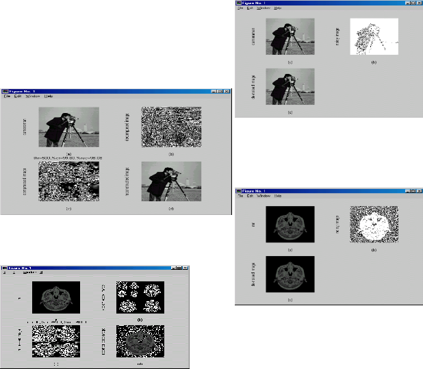
The snapshots of the implementation of Compres- sion & De-noising for different images are shown

Figure 8.3. (a) Input image(testpart) (b) Decomposed image

Figure 8.4. (a) Input image(cameraman)

(b) Noisy image (c) De-noised image .

Figure 8.1. (a) Input image(cameraman) (b) Decomposed

image (c) Compressed image (d) Reconstructed image.

Figure 8.5. (a) Input image(MRI) (b) Noisy image

Figure 8.2. (a) Input image(MRI) (b) Decomposed image (c)

Compressed image (d) Reconstructed image.

International Journal of Scientific & Engineering Research Volume 2, Issue 4, April-2011 7

ISSN 2229-5518

split.

Acknoweledgements

Authors thank Singhania University Rajastan and Vidya

Vikas Institute of Technology, Mysore.

Bibliography

Figure 8.6. (a) Input image(Testpart) (b) Noisy image (c) De- noised image.

9.Conclusion

The Slantlet transform orthogonal filterbank uses the filters of shorter length as compared to iterated 2- scale DWT filterbank. The number of filters increases according to the order. The Slantlet transform gives better compression result for the piecewise linear data. The Slantlet transform has been applied for compression and de-noising of various images. The matlab programs for the Slantlet transform applied for compression and de- noising are developed and the computer simulation is carried out for some test images. It is observed that as the threshold level increases better compression ratio and PSNR can be achieved for the test data.

10. Future scope

The present work can be extended to compare the performance of applying Wavelet transform and Slantlet transform on images and also study the characte- ristics/performance benefits of Slantlet transform over Wavelet transform. This work can be enhanced to wavelet packets, which offers a more complex and flexible analy-

sis, because the details as well as the approximations are

1. I. W. Selesnick, “The Slantlet Transform,” IEEE Transaction on signal processing, vol 47, No. 5, May 1999.

2. David l. Donoho “Smooth wavelet decomposi- tions with blocky coefficient kernels “ May, 1993.

3. Vaidyanathan, p. p., “Multirate systems and filter banks”, prentice hall inc., Englewood cliffs, new jersey, 1993.

4. M. Lmg, H. Guo, et. al “Noise reduction using an undecimated discrete wavelet transform”, IEEE signal processing , vol 3, no. 1, Jan 1996.

5. Aali M. Reza ,”From Fourier transform to Wave- let transform”, October 27, 1999 white paper.

6. Paolo Zatelli, Andrea Antonello, ” New Grass modules for multiresolution analysis with wave- lets”, proceedings of the open source gis - grass users conference, September 2002.

7. Kenneth Lee, Sinhye Park, et.al, “Wavelet-based image and video compression”, Tcom 502, April,

1997.

8. Dr. Guangyi Chen , ”Signal or Image denoising using wavelets, multiwavelets and curvelets”,

2004.