International Journal of Scientific & Engineering Research,Volume 3, Issue 6, June-2012 1
ISSN 2229-5518
Simulation of a Swarm Based Painting Algorithm
Animesh Kundu, Praneeth Talluri, Deepanwita Das
Abstract— This paper presents the simulation of a distributed algorithm for painting a priori known rectangular region [9] by swarm of mobile robots. The algorithm divides the whole region into some horizontal strips and each strip is assigned to a particular robot for
painting. The simulation is done with Player/Stage Robotic Simulation software. We have simulated an artificial environment that resembles the algorithm and studied the performance of the algorithm. The simulated result proves the correctness of the algorithm.
—————————— ——————————
warm of low cost mobile robots provides an attractive- facility of scanning any bounded region in a distributed manner. This facility can be applied for automated humani-
tarian demining, lawn mowing and milling, sweeping
[1], search and rescue of victims, terrain mapping, space
explorations, aerial reconnaissance etc.
In this paper, we concentrate on simulating an area cover-
age algorithm that is designed for painting a known rec- tangular region [9]. In this algorithm, we assume that a swarm of N robots are initially deployed within the given rectangular region. For simulating the algorithm using Player/Stage simulation software, we have designed a con- trol program to be executed by each of the robots. We as- sume that there is no central control over the robots and the robots do not communicate among themselves. The whole rectangular region which is to be covered is considered as a world. The basic idea of the algorithm is to partition the world into a number of non overlapping strips/cells and each cell is assigned to a distinct robot which will be re- sponsible for painting that particular cell. Based on the ini- tial locations of any robot and its neighbors, the robots calculates their ranks as well as the cell to be painted by it. In our simulation the robots rank themselves, calculating the final goal point and reach there to start painting. It is implied that on reaching the final goal point the robots will start painting and finish the job within finite amount of time.
This work takes root in the Boustrophedon decomposition
approach [4], which is an exact cellular decomposition,
where each cell can be covered with simple back-and-forth
motions like most of the related work on Multi robot cov- erage [5], [6], [7], [8], [9]. Together with that our simulated robots also follow the basic wait-observe-compute-move mod- el [3]
Due to space limitations we will briefly outline the major
approaches in multi-robot coverage (for a more detailed survey please refers to [9]).
Most of the previous works consider the presence of obstacles within the area to be covered. The algorithms are usually meant for single robot, which are further extended to team based multi-robot system [6], [7]. In the team based approach, communication, coordination and synchronization among the team members involves great complexity. In [8], authors used distributed approach but the robots are artificially deployed at fixed starting points located at regular intervals.
Moreover, the robots are also active in every cycle. Task re-
allocation requires complex and accurate cost estimation
and localization. In [5] and [8], maintaining the graphs
requires large amount of memory.
In this paper, we have simulated the algorithm proposed in
[9], which is based on a more stronger model than the re- lated works. This algorithm is based on asynchronous model
[2]. It is theorically proved that the algorithm is correct. Our simulation proves the correctness of the algorithm in a simulated environment that is similar to any practical situ- ation.
Our aim is to simulate the robots to paint a given rectangular region by them. Robots may occupy any position within the region. We assume that no two robots occupy the same posi- tion. The robots are relatively weak, simple and assumed to have the following characteristics [3]:
1. Identical and Homogeneous - All the simulated robots are identical in all respect, specially, they have the same computational capability. All the robots are assumed to be point robots with unlimited visibility. However, we assume that each of them is having a sensing zone of radius T (T is small)[9].
2. Computational Model - Here we follow the basic Observe-Compute-Move [3] model. A computational cycle is defined to be a sequence of “observe”, “compute” and
IJSER © 2012
International Journal of Scientific & Engineering Research,Volume 3, Issue 6, June-2012 2
ISSN 2229-5518
“move” steps. Each of the robots executes same instructions in all the computational cycles. Once a robot completes one computational cycle, it starts executing the next one. The ac-
tions taken by a robot in “compute” and “move” steps, entirely depend on the observations made in “observe” step. In some situations, an observation might lead a robot not to change its position in “move” step. In such cases the robot seems to be idle, though it is actually executing all the three steps.
3. Oblivious or Memoryless - Robots do not retain any information gathered in the previous computational cycle.
The “painting” operation considered here is assumed to be an Atomic operation. That means, the painting step would be completed uninterruptedly.
The models considered here are as follows:
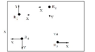
of variable lengths. They do not share any common clock [2].Direction only: Directions of both axes are common to all the robots, but the positive orientation of the axes may be dif- ferent [2]. Here, we assume that x-axes of the robots are paral- lel to the known common reference line. Therefore, the direc- tion of x-axis is common to all the robots but the robots may have different views of the positive orientation of the axis. However, it is assumed that the direction of the positive y-axis is 90_ counterclockwise to the positive direction of the x-axis. Each robot has its local co-ordinate system. All the robots would assume that they occupy the position (0; 0) with respect to their local co-ordinate system. Further, we assume that
these various co-ordinate systems might not share a common
scale. Figure 1 shows the local co-ordinate systems of four ro- bots
R1, R2, R3, and R4, and the common reference line
XX
————————————————
Fig. 1. Positive orientation of the local axes of R1 and R3 are just the reverse of that of the robots R2 and R4
The first sub-section describes the proposed algorithm. All the observations supporting the correctness of the Algorithm are listed in the second sub-section, however for the proofs refer
to [9]. The simulation of the algorithm is discussed in the next section.
It is assumed that the region, to be painted is a rectangular region and no obstacles are there within the region. Futher,we assume that all the N robots are enclosed within the region. Without loss of generality, we assume that the common reference line be parallel to one side of the rectan- gular region.
As soon as a robot R becomes alive it performs the follow-
ing computational cycle “observe-compute-move”. As
long as a robot is in alive state, after completing one such computational cycle, it would again start another cycle and continue in this way until it completes its assigned job. Algorithm Paint: (executed by a robot R) We have designed a control program that has to be executed by each of the robots in the simulation environment. The controller controls differ- ent parts of any robot and enables them to execute the below mentioned phases. Observe According to the local co-ordinate system, the robot R first observes the positions of all other ro- bots. Let the co-ordinates of other robots be (a1; b1), (a2; b2),…, (aN-1; bN-1), whereas, its own co-ordinate would be (0; 0). It is to
be noted here that some of these ai, bi values might be negative
also. This phase will be executed by using a laser and a blob- finder [10].
Step 1:
According to the values of y-co-ordinates, the robot R will or-
der all the robots (including itself) so that the robot having the largest value of y co-ordinate will have the highest rank, that is, N. Without loss of generality, we assume that after sorting the co-ordinates of N robots are (x1; y1), (x2; y2), …, (xN; yN), so that y1 _ y2 _ y3…. yN. The robot having the co-ordinate (xi; yi)
IJSER © 2012
International Journal of Scientific & Engineering Research,Volume 3, Issue 6, June-2012 3
ISSN 2229-5518
would have the rank i and the robot will be mentioned as Ri, 1
_ i _ N. In case of a tie, the values of x -co-ordinate of the ro-
bots are to be considered. The robot having lower x-co-
ordinate would have the lower rank. As we have assumed that no two robots can occupy the same position, two robots hav- ing the same y-co-ordinate cannot have identical x-co-ordinate also. In this way, the robot R would determine its own rank.
Let the rank of R be k. From now on R and Rk will be used
interchangeably. Step 2:
According to the local co-ordinate system of R, let the upper boundary of the region to be painted be at a vertical distance
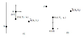
Fig. 2. Secondary destinations w.r.t robot R
s and the lower boundary be at f. Since all the robots are en-
closed within the area, s >=0 and f <= 0. The whole rectangular area will be divided into N equal horizontal strips of height ( (s-f)/ N ). The top most (according to the local co-ordinate sys- tem of R) strip will be considered as the Nth strip and the bot- tom most one will be considered as thefirst strip. Now the ro-
bot Rk will identify the kth strip by computing its upper and lower boundary as f+(k-1)*( (s-f)/ N ) and f +k *( (s-f)/N ). The kth strip will be colored by Rk. Each robot would start the co- loring from the bottom left corner of the assigned strip. Ac- cordingly the robot would compute its destination.
On the way towards their destination, robots would maintain
their relative ranking. It means, while moving, robots should not cross vertically any other robot even if their routes do not
intersect each other. In other words, to reach the destination, if a robot is going to gain a vertical height higher (lower) than a robot of higher(lower) rank (that is, it is crossing another robot which would affect the relative ranking), it would stop at an _ (pre-defined small quantity) distance from that height and would wait for that other robot to move on.
Due to the rule stated above, the robot R may need to take a
halt before reaching its final destination i.e.; the bottom-left corner of the assigned strip. In this compute step, the robot R should verify this situation and if required, it would recalcu- late the position of the halt. We call this as the secondary desti- nation. Suppose, to reach the final destination, R has to verti-
cally cross another robot R which is at a point (x1, y1). Accord- ing to the given rule, R would stop at a vertical height of y1 ... Therefore, the modified destination of R would be (0, y1 ..). Figure 2 shows two possible cases. In Figure 2(a), to reach the destination D, the robot R has to move in the vertically downward direction and then it requires to cross R (which is
of lower rank). Therefore, the secondary destination of R
would be D’(0, y1+є). In Figure 2(b), to reach the destination D, the robot R has to move in the vertically upward direction and then it requires to cross R (which is of higher rank in this case). Therefore, its secondary destination would be D’(0, y1-є).
After identifying the assigned strip, the robot would start moving towards its destination point, the bottom left corner point of the assigned strip. Actually the robots do not need to reach the exact position of its destination due to its sensing ability. It is sufficient to reach a height, which is at a distance T(above/below) away from the final destination. It is to be noted here that, though the final destination of a robot is the bottom left corner point of the assigned strip, sometimes, to preserve the relative ranking, robots may need to wait at cer- tain height for some other robot to move on. A robot would always move in vertical direction first, after acquiring the ver- tical height of the final destination, the robot would then move into horizontal direction to reach the final destination. Thus, to reach the secondary destination, a robot moves only in vertical direction. Depending on whether a robot reaches its final or secondary destination, the following two courses of actions would be taken by the robot:
(i) As soon as, a robot reaches the secondary destination,
this “move” state terminates. That is, the computational cycle
will be terminated and the robot will again start a new compu- tational cycle with “observe” state.
(ii) Once the robot reaches its final destination, before starting the painting, it would check whether there is any other robot present in its assigned strip. If not, it would start painting the assigned area. It would complete the job successfully, without any interruption and at the end, it would generate a signal that its job is done. Otherwise, if the robot R finds another ro- bot, say R, present in its assigned strip, it would terminate the computational cycle at that moment. That is, here also the ro- bot would wait for that other robot to move on. At any point
of time, if the robot R finds another robot R at the same vertic-
al height (which might occur at the starting time, if initially they are at the same height), then depending on the rank of R and that of itself, R decides its next course of action as follows: Case A : The rank of R is greater than that of R and th destina- tion of R is in its positive direction.
Case B : The rank of R is less than that of R and the destination of R is in its negative direction.
IJSER © 2012
International Journal of Scientific & Engineering Research,Volume 3, Issue 6, June-2012 4
ISSN 2229-5518
For both the cases, R would break the tie and would move first towards its destination point.
Case C : The rank of R is greater than that of R and the desti- nation of R is in its negative direction.
Case D : The rank of R is less than that of R and the destination
of R is in its positive direction.
For both the cases R will wait for R to move first towards
its destination point.
of the robots computed by several robots are same upto a reversal of order. In other words, if the robots R1 and R2 compute the rank of a robot R as i and j respectively, then either i = j or i = N + 1 � j and this would remain same throughout the algorithm.
to the robots remains invariant with respect to any
computational cycle.
the robots a non-conflicting decision regarding tie-breaking. Observation 5: The process would start within finite amount of time.
time.
The simulation has been performed using Player / Stage robot- ic simulation software. Player / Stage provides facilities to model the robots, design the environment and simulate auto- nomous systems [10]. Player is the program implementing the algorithm for distributed robotic control based on TCP/IP and
802.11 wireless ethernet. Stage is a graphical user interface that
supports an environment for simulation using robots, sensors and obstacles. To simulate any algorithm we need to configure the properties of the robots in the swarm, design the environ- ment where the robots will be deployed (Stage) and execute
the controller program (Player). Player and Stage works simul-
taneously to simulate the algorithm
The robots used in the simulation of the above mentioned al- gorithm have a dimension of 1 x 1 x 1, colored green and are equipped with the following devices :
![]() Infrared Laser sensors : Range - 20 units, 180 scan
Infrared Laser sensors : Range - 20 units, 180 scan
lines, 180 degree field of view, 180 samples.
![]() Blobfinder : Colors recognized - 2 (red and green),
Blobfinder : Colors recognized - 2 (red and green),
160x 120 image size, 20 range, 180 degree field of
view.
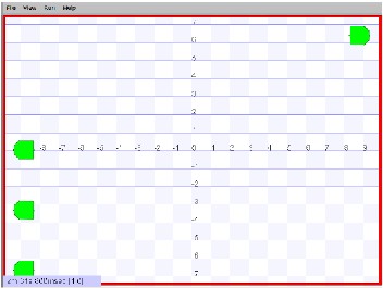
The simulation environment is constructed with a 16 units x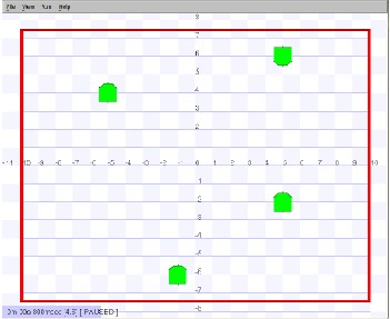
21 units. Figure 3 shows the world with four robots. The boundary which encloses the map is colored red. The robots are placed randomly on the map.
Fig 3: A world with four robots
The program implementing the algorithm is written in C++. It uses the libplayerc++ library to communicate with Stage. It performs the look, compute and move steps in accodance
with the algorithm. Figure 4 shows some portion of the code.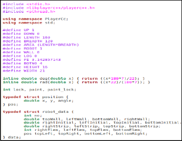
Fig 4: Some portion of the code
Ubuntu 10.04 (Lucid Lynx) is used as the platform for
IJSER © 2012
International Journal of Scientific & Engineering Research,Volume 3, Issue 6, June-2012 5
ISSN 2229-5518
simulation of the algorithm with hardware specification [ RAM : 2.00 GB, intel core2duo processor with 3.00 GHz]. Four identical robots has been used in the simulation. The robots
have successfully observed each other, calculating their rank dynamically, deciding the strip to be painted by it and moving to the final goal point. Based on the random placement of the 4 robots on the map, mainly three different cases were simu- lated and these do not include the cases, where more than two robots are in a straight line. We have simulated 5 such tests for each of the case.
![]() case I: All the robots are having same orientation.
case I: All the robots are having same orientation.
Average time taken to reach the goal point for the 5 tests is 2 minutes 33 seconds.
![]() case II: Robots may have opposite orientations. Av-
case II: Robots may have opposite orientations. Av-
erage time taken to reach the goal point for the 5 tests is 2 minutes 30 seconds.
![]() case III: Robots (2) are on the same line and having
case III: Robots (2) are on the same line and having
opposite orientations. Average time taken to reach the goal point for the 5 tests is 2 minutes 25 seconds.
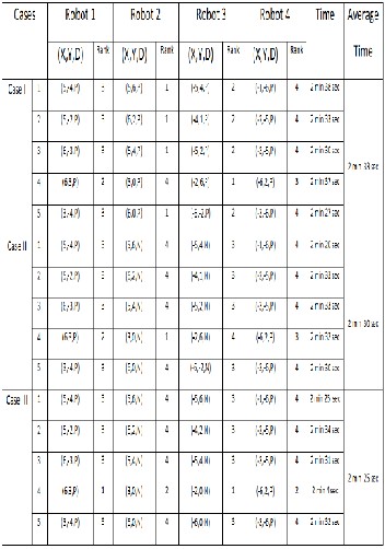
It is implied that once a robot reaches its goal point, it will
complete the painting by following simple back and forth mo- tion. We have considered the total time taken by all robot to reach their goal point before the starting of actual painting. Due to space constraints all the cases cannot be included, only some of the cases and their results are shown in Figure 5. In Figure 4, X,Y refer to the coordinates of the robot and D refers to orientation of the robot that is P for positive orientation, N for negative orientation.
IJSER © 2012
International Journal of Scientific & Engineering Research,Volume 3, Issue 6, June-2012 6
ISSN 2229-5518
where more than two robots are placed in the same straight line..
Fig5: Results of the cases
Figure 6 indicates the final goal points reached by the ro- bots.The results obtained from the simulation are coherent with the theoretical proofs.
Fig 6:Final Goal points reached by the robots
In this paper, we have simulated a distributed algorithm for painting a priori known rectangular region by a swarm of N robots, each having their local co-ordinate system. This algo- rithm is based on direction-only and Asynchronous model.
The algorithm guarantees complete coverage within a finite- time. Algorithm Paint can also be used for painting any Fig. 6. Final goal points reached by the robots polygonal region, pro- vided the region is convex. However, in that case, though all the strips would have the same height, their area will be dif- ferent and thus the assigned job of each robot may not be equal. For future work, we would like to extend the algorithm
[1] D. Kurabayashi, “Cooperative sweeping by multiple mobile robots,” in IEEE Int. Conf. on Robotics and Automation, vol. 2, pp. 1744 1749, Min- neapolis, USA, April 1996.
[2] A. Efrima and D. Peleg, “Distributed algorithms for partitioning a
swarm of autonomous mobile robots,” Technical Report MCS06- 08, The
Weizmann Institute of Science, October 2006.
[3] P. Flochinni, G. Prencipe, N. Santoro and P. Widmayer, “Distributed
coordination of a set of autonomous mobile robots,” In
Proc. IEEE Intelligent Vehicles Symp, 2000, pp. 480-485.
[4] H. Choset and P. Pignon, Coverage path planning: The boustrophe- don cellular decomposition, in Int. Conf. on Field and Service Robotics, Canberra, Australia, 1997.
[5] C. Kong, N.A. Peng and I. Rekletis, “Distributed coverage with multi-robot system,” in IEEE Int. Conf. on Robotics and Automation, Orlando, USA, pp. 2423-2429, June 2006.
[6] I. Rekletis, V. Lee-Shue, A.P. New and H. Choset, “Limited communication, multi-robot team based coverage,” in IEEE Int. Conf. on Robotics and Automation, Orleans, LA, pp. 3462-3468, April 2004.
[7] D. Latimer, S. Srinivasa, V. Lee-Shue, S. Sonne, H. Choset and A.
Hurst, “Toward sensor based coverage with robot teams,” in IEEE Int. Conf. on Robotics and Automation, Carnegie Mellon Univ., Pittsburgh, PA, vol.1, pp. 961-967, August 2002.
[8] I. Rekletis, A.P. New, E.S. Rankin and H. Choset, “Efficient
boustrophedon multi-robot coverage: An algorithmic approach,”
Annals of Mathematics and Artificial Intelligence, vol. 52(2-4), pp. 109-142,
2008.
[9] D. Das and S. Mukhopadhyay, “An Algorithm for Painting an Area by Swarm of Mobile Robots ,” Int. Conf. on Control, Automation and Robotics, Singapore, pp. C1-C6, Feb 2011.
gence, vol. 52(2-4), pp. 109-142, 2008.
[10] B. P. Gerkey, R. T. Vaughan, and A. Howard. “The player/stage project: Tools for multi-robot and distributed sensor systems,” Int. Conf. on Advanced Robotics, pp. 317-323, Feb 2003.
IJSER © 2012