International Journal of Scientific & Engineering Research Volume 4, Issue 1, January-2013 1
ISSN 2229-5518
Simulation analysis of various PID controller algorithms and their impact on design of Anti Lock Brake
Dileep Kumar Bhoi, Devesh Singh Patel, Premananda Sahoo
In this paper we are not discussing on the tuning aspect of PID controller but on the basic design configurations of various P-I-D and their impact on design of Antilock Brake (ABS) as a case study .There are three basic design approaches for a PID controller: Ideal, Parallel and Series. These three configurat ions are separately studied by using them as an Antilock Brake Controller and their impact on st opping distance and stopping time is analyzed.
Stopping distance is the dist ance travelled by the vehicle after applying the brake and time for the vehicle t o reach to complete halt is stopping time. We can, in general consider a controller as a good controller if it helps to reduce both st opping distance and tim e.
Under the influence of Drive torque, the vehicle moves and due to air drag, braking torque, surface friction and inertia, vehicle com e to stop. A dynamic com bination of all these torques and forces are responsible for motion of vehicle on a surface and coefficient of
friction between tyre and road-surface, am ount of steering etc contribute further to vehicle dynamics.
Due to drive torque generat ed by engine, the wheels starts rotating and when brake applied it comes to halt after sometime.
Vehicle speed and wheel angular speed are proportional in normal condition but when hard braking is made it is possible that vehicle speed is
not slowing down at the sam e rat e as wheel angular speed, causing the slip.
Slip is a situation created by locking of wheels, m eans wheels not rotating but vehicle is m oving. This is a fatal driving condition and driver can lose the control of vehicle and the time to st op the vehicle increases.
—————————— ——————————
The influence of individual elements on the characteristic of a
PID controller is summarized below:
Closed Loop Response | Rise Time | Overshoot | Settling Time | Steady- State Error |
P | Decrease | Increase | Small Change | Decrease |
I | Decrease | Increase | Increase | Eliminate |
D | Small Change | Decrease | Decrease | Small Change |
Although from implementation point of view, PID controller seems easier but tuning it to an appropriate combination is very tedious job and this is the exact reason which gives scope of developing several tuning algorithms. Particularly
for complex mechanical system with certain lag or hysteresis,
A good control system should ideally have smaller rise time, less overshoot, smaller settling time and steady state error. So having a combination of P, I and D in such a way that an ideal controller design can be obtained using any generic empirical formula; unfortunately does not exist.
A design tuned for any particular application may be completely unsuitable in other scenario.
When we speak about a PID, it’s not a unique design but has three basic approaches. There are three configuration of PID controller: Ideal, Series and Parallel [2].
In time domain, these three configurations are defined as below:
the PID controller does not yield good result due to non- linearity.
u(t)=K c e(t) +
![]()
1
I ∫ e(t)d(t) + D
![]()
de(t) ......equation(1)
dt
IJSER © 2013 http://www.ijser.org
International Journal of Scientific & Engineering Research Volume 4, Issue 1, January-2013 2
ISSN 2229-5518
![]()
1
u(t) = KP [e(t)] + I ∫ e(t)d(t) + D
1
![]()
de(t) .......equation (2)
dt
d
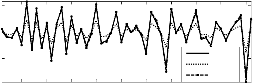
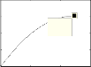
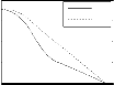
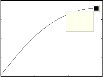
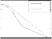
These three types of PID design approaches were subjected to standard step input and uniform random signal, their response obtained is shown in Figure 4 and Figure 5
respectively.![]()
![]()
u(t) =Kc e(t) + I ∫ e(t)d(t) 1 + D dt ......equation (3)
Where, u(t) is the input signal to the plant model, the error
For reference, an On-Off (Bang-Bang) controller is used. Output of On-Off controller is having just two levels saturated to limits and is easiest to implement.
signal e(t) is defined as e(t) =r(t) − y(t), and r(t) is the reference input signal.
KC and KP are gain, I is integral and D is derivative component.
1
0.8
0.6
0.4
0.2
0
Error Signal e(t)

10 20 30 40 50
1
0.8
0.6
0.4
0.2
0
Output with On-Off Controller

10 20 30 40 50
Output with Different PID algorithms
The controller design of three PID approaches described above is given below in Figure 1, 2 and3 respectively. Design is done using SIMULINK blocks and equations (1) through (3) described above.
For simulation, fixed step solver ode1(Euler) type is used.
Ideal
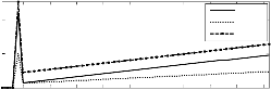
40 Parallel
Series
20
0
5 10 15 20 25 30 35 40 45 50
Error Signal e(t)
Output with On-Off Controller

1

1
0
-1
-2
10 20 30 40 50
0.5
0
-0.5
-1
10 20 30 40 50
100
0
-100
Output with Different PID algorithms
Ideal
Parallel
Series
5 10 15 20 25 30 35 40 45 50
To determine suitability of any particular PID approach, we
have considered its potential application in antilock brake system.
Due to non linearity in vehicle model and controller algorithm, tuning it for all kind of road situation is very difficult and various studies ongoing to find an optimal
IJSER © 2013 http://www.ijser.org
International Journal of Scientific & Engineering Research Volume 4, Issue 1, January-2013 3
ISSN 2229-5518
solution. Although, we are just trying to assess suitability of a basic PID approach in this study; without going in the discussion of any such algorithms in particular.
In Figure 6, we have constructed a SIMULINK model of vehicle (plant model) and derived wheel speed and vehicle
speed and subsequently stopping distance.
Stopping distance is the figure of merit for our analysis, although smaller stopping distance is not the only objective of any ABS but controllability of vehicle is equally important during hard braking.
Computation of wheel and vehicle speed’s angular component, slip and stopping distance is explained in
subsequent sections.
Angular velocity is calculated as [12]:
![]()
t =
- - . Ft - .F
………….equation(4)
Or , = ∫
- - . Ft - . F
t ….equation(5)
Where, ω is angular velocity, Td is torque generated by engine(in Nm), Tb is torque produced by pressing brake pedal(in Nm), Rw is radius of wheel(in m), Ft is traction force(in N) ,Fw is wheel viscous friction(in N).
The, traction force is given by [12],
As we know, that to ensure correct analysis ,a good representative model of the process/plant (in this case vehicle model) is required, so going by classical control system theory, we here developed a plant model of a vehicle.
Ft = µ(λ). N = µ .M .g .....equation (6)
Where, µ is coefficient of friction between tyre and road surface, M is the mass component of the vehicle acting on a wheel and theoretically it is quarter of total mass of the vehicle.
Vehicle speed is given by
To evaluate the various controller algorithms which could be used in design of antilock brake, we have used a plant model of a vehicle which under the influence of drive torque
V
t =
N Ft - Fv
M .............equation (7)
produces angular velocity in the wheels and linear velocity of the vehicle.
Or, V = ∫ N Ft - Fv M
.............equation (8)
Due to the friction we always find difference in angular velocity of wheel and vehicle velocity which is known as slip.
The basic forces acting on vehicle are: drive torque as a response to gas pedal pressed and brake torque and steering applied by driver .Combination of these three forces give direction and movement to the vehicle.
Consider a wheel resting and rotating in contact with ground
Where, Nw is number of wheels, Fv is air drag force and M is mass of vehicle.
Vehicle angular velocity ωv is given as
ωv=V/Rw .................................................equation (9) And wheel slip is defined as
surface as shown in Figure 7.![]()
ww -wv
=
w , v
.....................................equation (10)
IJSER © 2013 http://www.ijser.org
International Journal of Scientific & Engineering Research Volume 4, Issue 1, January-2013 4
ISSN 2229-5518
Using equation (4) through (10), we derive stopping distance achieved by using various PID approaches in subsequent
sections.
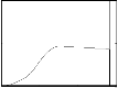
(A)Wheel Speed & Vehicle Speed
80
Ww
(B)Slip Ratio

1
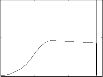
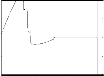
As shown in Figure 6, we connected various PID controller strategies one by one and after running the simulation, results are obtained.
The desired slip ratio is kept 0.2 and PID controllers as shown in Figure 1,2 and 3 are connected keeping all other parameters unchanged.
60 Wv
40
20
0
0 5 10 15
Time
(C)Output of Controller

2
1
0
-1
-2
0 5 10 15
Time
0.5
0
800
600
400
200
0
0 5 10 15
Time
(D)Stopping Distance
X: 12.33
Y: 606.5
0 5 10 15
Time
(A)Wheel Speed & Vehicle Speed
80
Ww
(B)Slip Ratio
1
60 Wv
40
20
0
0 5 10 15
Time
(C)Output of Controller
2
1
0
0.5
0
800
600
400
0 5 10 15
Time
(D)Stopping Distance
X: 14.16
Y : 713.4
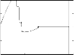
Two most important parameters: Stopping distance and stopping time of vehicle are summarized below:
-1
-2
0 5 10 15
Time
200
0
0 5 10 15
Time
We can conclude that performance of ideal and parallel configurations are marginally different i.e. same stopping
(A)Wheel Speed & Vehicle Speed
80
Ww
(B)Slip Ratio
1
distance is obtained but the time required to fully stop is less in case of parallel configuration(14.01 sec against
60 Wv
40
20
0
0 5 10 15
Time
(C)Output of Controller
2
1
0
-1
-2
0 5 10 15
Time
0.5
0
800
600
400
200
0
0 5 10 15
Time
(D)Stopping Distance
X: 14.01
Y: 713.4
0 5 10 15
Time
14.16 sec).
But, the series configuration has distinct advantage over other two configurations, as we see reduction in both stopping distance and stopping time.
By analysing the results it can be safely concluded that in application like ABS where quicker stopping of vehicle is crucial, use of series configuration of PID could be
recommended. After having designed a PID with series
IJSER © 2013 http://www.ijser.org
International Journal of Scientific & Engineering Research Volume 4, Issue 1, January-2013 5
ISSN 2229-5518
configuration,performance could be further enhanced by carefully selecting Kc,Kp,I and D values.
Ziegler Nichols or Cohel-Coon tuning methods could be additionally used to get a better stopping distance or shorter stopping time.
Authors wish to thank their organization Continental
Automotive GmbH.
[1] Dingyu Xue, YangQuan Chen, and Derek P. Athert on, “Linear
Feedback Control ”.
[2] Karl J. A . Strom, Pedro Albertos, and Joseba Quevedo, “PID Control” ,Control Engineering Practice 9 (2001) 1159–1161
[3] Majed Hamdan, “Modified PID Control of Pneumatic Valves wit h Hysteresis”, M.S. Thesis, Departm ent of Electrical Engineering, Cleveland St ate University, April 1997
[4 ] Bernard Friedland, “Advanced Control System Design”, New
Jersey: Prentice Hall, 1996]
[5] P. E. W ellst ead, “Analysis and Redesign of an Antilock Brake
System Controller,” IEEE Proceedings Control Theory Applications, Vol.
144, No. 5, September 1997, pp. 413-426.
[6] D. Cho and J. K. Hedrick, “Automotive Powertrain Mod-eling for Control,” Transactions ASME Journal of Dy-namic System s, Measurem ents and Control, Vol.111, No.4, December 1989, pp. 568-
576.
[7] Y. K. Chin, W. C. Lin and D. Sidlosky, “Sliding-Mode ABS W heel
Slip Control,” Proceedings of 1992 ACC, Chicago, 1992, pp. 1-6.
[8] C. Jun, “The Study of ABS Control System with Differ-ent Control Methods,” Proceedings of the 4th Interna-tional Symposium on Advanced Vehicle Control, Nagoya, 1998, pp. 623-628.
[9] S. Solyom, “Synthesis of a Model-Based Tire Slip Con-troller,” Synthesis of a Model-Based Tire Slip Controller, Vol. 41, No. 6, 2004, pp. 475-499.
[10] W. Ting and J. Lin, “Nonlinear Control Design of Anti-lock Braking Systems Com bined with Active Sus-pensions,” Technical Report of Department of Electrical Engineering, National Chi Nan University, 2005.
[11] A. A. Aly, “Intelligent Fuzzy Control for Antilock Brake System with Road-Surfaces Identifier,” 2010 IEEE In-ternational Conference on Mechatronics and Aut omation, Xi’an, 2010, pp. 2292-2299.
[12]http://scholar.lib.vt.edu/theses/ available/etd5440202339731121/unre stricted/CHAP3_DOC.pdf
IJSER © 2013 http://www.ijser.org