International Journal of Scientific & Engineering Research, Volume 4, Issue 8, August-2013 14
ISSN 2229-5518
Sequential Intrusion Detection System Using Distance Learning (Metric Learning) and Genetic Algorithm
Ezat soleiman, abdelhamid fetanat
—————————— ——————————
He insufficiency of traditional security tools like antivirus in facing current attacks conducts to the development of intrusion detection systems (IDS). IDSs search in the net- work traffic for malicious signature and then send an alarm to the user. Since current IDSs are signature based they still una- ble to detect new forms of attacks even if these attacks are slightly derived from known ones. So, recent researches con- centrate on developing new techniques, algorithms and IDSs that use intelligent methods like neural networks, data min-
ing, fuzzy logicm and genetic algorithms.
Genetic algorithm is an evolutionary optimization technique based on the principles of natural selection and genetics. The working of genetic algorithm was explained by John Holland [1]. It has been successfully employed to solve wide range of complex optimization problems where search space is too large. GA evolves a population of initial individuals to a population of high quality individuals, where each individual represents a solution of the problem to be solved. Each indi- vidual is called a chromosome, and is composed of a prede- termined number of genes. The quality of fitness of each chromosome is measured by a fitness function that is based on the problem being solved. The algorithm starts with an initial population of randomly generated individuals. Then the pop- ulation is evolved for a number of generations while gradually improving the qualities of the individuals in the sense of in- creasing the fitness value as the measure of quality. During each generation, three basic genetic operators are applied to each individual with certain probabilities, i.e. selection (rank selection, roulette wheel selection and tournament based selec- tion), crossover and mutation.
There are many parameters to consider for the application of GA. Each of these parameters heavily influences the effective- ness of the genetic algorithm [2].
The fitness function is one of the most important parameters in genetic algorithm. To evolve input features and network structure simultaneously, the fitness, which is based on the detection accuracy rate, includes a penalty factor for the num- ber of operative input nodes and a penalty factor for the num- ber of operative hidden nodes.
In mathematics, there are multiple feature spaces that are useful in enormous problems. For example, Euclidian space or Euclidian distance is the most popular metric that we use in our real world or Mahalanobis distance that we use to demon- strate the distance between two places in the city.
In classification and clustering problems, the majority of methods, assumes the Euclidian feature space to solve their problems and they evaluate their result in this space. One question may appear in mind is what is the best feature space for my problem? In other words, is this distance metric the best metric for my problem? In the next section we discuss about it with some example.
Based on figure 1, suppose Ali, Mohammad and Hasan were Arab and Bryan, David and Michel were American. If we want to classify them based on Euclidian distance between
their houses, Ali should be American because Ali’s house is
• Ph.D. Candidate, Dept of ICT Eng, Maleke Ashtar Univ. of Tech., Islamic
Republic of Iran. Email: ezut_sol73@yahoo.com
• Assistant Professor, Maleke Ashtar Univ. of Tech, Islamic Republic of
Iran. Email: abfetanat@gmail.com.
next to Bryan’s house and this scenario is the same with Mo- hammad-David and Hasan-Michel. So in this classification problem, Euclidian distance is not useful. Note that Euclidian distance is meaningful but is not useful.
IJSER © 2013 http://www.ijser.org
International Journal of Scientific & Engineering Research, Volume 4, Issue 8, August-2013 15
ISSN 2229-5518
![]()
![]()
![]()
![]() T
T
Ali Mohammad Hasan
![]()
![]()
![]()
Fig. 4.
Bryan David Michel
Fig. 1.
Is there any transform so that if we transform their house location, in transformed space, the Euclidian distance demon- strates their class?![]()
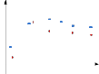
Suppose we have found a transform and transformed loca- tions were figure 2.![]()
![]() David
David
![]()
![]()
Ali ![]()
Mohammad
Michel
Bryan
Hasan
Fig. 2.
In this space, Euclidian distance is useful and it properly helps us to classify them based on Euclidian distance.
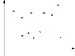
Another example is in intrusion detection systems. Suppose
We will use LMNN method for metric learning. This method has shown its strength in classification problems. In the next section we will introduce it.
Large margin nearest neighbor (LMNN) classification is a statistical machine learning algorithm. It learns a Pseudo metric designed for k-nearest neighbor classification. The algorithm is based on semi definite programming, a sub-class of convex op- timization [3].
The goal of supervised learning (more specifically classifi- cation) is to learn a decision rule that can categorize data in- stances into pre-defined classes. The k-nearest neighbor rule assumes a training data set of labeled instances (i.e. the classes are known). It classifies a new data instance with the class ob- tained from the majority vote of the k closest (labeled) training instances. Closeness is measured with a pre-defined metric. Large Margin Nearest Neighbors is an algorithm that learns this global (pseudo-)metric in a supervised fashion to improve the classification accuracy of the k-nearest neighbor rule [4].
The main intuition behind LMNN is to learn a pseudo met- ric under which all data instances in the training set are sur- rounded by at least k instances that share the same class label. If this is achieved, the leave-one-out error (a special case of cross validation) is minimized. Let the training data consist of a data set
(x , x )
each connection has two features 1 2 , for example
D = {(x , y ), ..., (x , y )} ⊂ R d ×C
(1)
(dst_host_srv_serror_rate,src_byte). In figure 3, suppose blue squares were normal connection and red circles were attack
connections.
, where the set of possible class categories is
C = {1,...,c}
The algorithm learns a pseudo metric of the type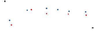
d (x , x
) = (x
− x
)T M (x
− x )
i j i j i j
. (2)
Fig. 3.
If the classification method was KNN, this input samples will produce high error rate because the intra class distances are high and inter class distances are low. If we find a transform T so that it reduces the intra class distance and increases the inter class distance, we can use KNN with low error rate.
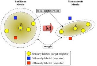
For d (., .) to be well defined, the matrix M needs to be pos- itive semi-definite. The Euclidean metric is a special case, where M is the identity matrix. This generalization is often (falsely) referred to as Mahalanobis metric.
Figure 5 illustrates the effect of the metric under varying M. The two circles show the set of points with equal distance to
x
the center i . In the Euclidean case this set is a circle, whereas
under the modified (Mahalanobis) metric it becomes an ellip- soid.
IJSER © 2013 http://www.ijser.org
International Journal of Scientific & Engineering Research, Volume 4, Issue 8, August-2013 16
ISSN 2229-5518
x i to be one unit further away than target neighbors x i
(and
x
therefore pushing them out of the local neighborhood of i ).
The resulting inequality constraint can be stated as:
∀i , j ∈ N i , l , y l
≠ y i
d (x , x ) +1 ≤ d (x , x ) + ξ
(4)
Fig. 5. Schematic illustration of LMNN.
The margin of exactly one unit fixes the scale of the matrix
M. Any alternative choice c > 0 would result in a rescaling of
1
![]()
M by a factor of c .
The final optimization problem becomes:
The algorithm distinguishes between two types of special da-
min ∑
d (x , x ) +
∑ ξijl
ta points: target neighbors and impostors.
M i , j ∈N i i , j ,l
∀i , j ∈ N i , l , y l
≠ y i
(5)
Target neighbors are selected before learning. Each instance
d (x , x ) +1 ≤ d (x , x ) + ξ
x i has exactly k different target neighbors within D, which all
y
shares the same class label i . The target neighbors are the
data points that should become nearest neighbors under the
ξijl
≥ 0 ,
M ≥ 0
(6)
learned metric. Let us denote the set of target neighbors for a
Here the slack variables
ξijl
absorb the amount of viola-
x N
data point i as i .
tions of the impostor constraints. Their overall sum is mini-
mized. The last constraint ensures that M is positive semi- definite. The optimization problem is an instance of semi defi-
nite programming (SDP). Although SDPs tend to suffer from
x x
An impostor of a data point i is another data point i with
high computational complexity, this particular SDP instance
y
a different class label (i.e. i
≠ y j ) which is one of the k
can be solved very efficiently due to the underlying geometric properties of the problem. In particular, most impostor con-
x
nearest neighbors of i . During learning the algorithm tries to
minimize the number of impostors for all data instances in the
training set.
Large Margin Nearest Neighbors should optimize the ma-
x
trix M. The objective is twofold: For every data point i , the
target neighbors should be close and the impostors should be far away. Figure 3 shows the effect of such an optimization on
an illustrative example. The learned metric causes the input
straints are naturally satisfied and do not need to be enforced during runtime. A particularly well suited solver technique is the working set method, which keeps a small set of constraints that are actively enforced and monitors the remaining (likely satisfied) constraints only occasionally to ensure correct- ness[5].
Our proposed algorithm has overall structure in figure 6.
vector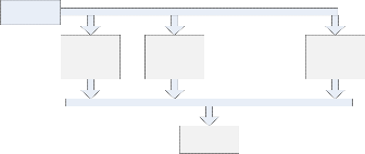
x i to be surrounded by training instances of the same
class. If it was a test point, it would be classified correctly un- der the k = 3 nearest neighbor rule.
The first optimization goal is achieved by minimizing the average distance between instances and their target neighbors
KDD dataset
IDS 1 IDS 2 IDS M
∑
i , j ∈N i
d (x i , x j )
(3)
Voting
The second goal is achieved by constraining impostors
Fig. 6.
IJSER © 2013 http://www.ijser.org
International Journal of Scientific & Engineering Research, Volume 4, Issue 8, August-2013 17
ISSN 2229-5518
The KDD data set are passed to each intrusion detection system and voting algorithm is used to make decision based on each IDS system result. Each IDS has same structure that we will explain in next section.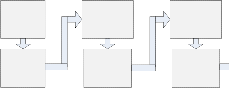

IDS has two phases: The train phase and test phase. In train phase, we sample from train data frequently and in each sam- pling, we change the selection probability of samples. Figure 7 illustrates the training phase.
This procedure will be continued until Nth learner is trained.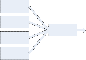
Each IDS will predict the label of each sample as attack connection or normal connection with some certainty. In the voting part of figure 6, we use genetic algorithm to make final decision. As you see in figure 8, we assign a weight to each IDS result.
IDS 1
KDD train data
IDS 1
IDS 2
IDS N
Sampling with equal probability
Sampling with non equal probability
Sampling with non equal probability
Fig. 7.
IDS 2
IDS 3
∑w i pi P
If D = (d1 , d 2 ,..., d n )
and
S = (s1 , s 2 ,..., s k )
were the
IDS M
training set and samples set respectively, at the first step, each
1
![]()
sample has equal probability n . We sample k samples from train data and pass them to metric learner 1. Then we learn the learner and at the next step we decrement the probability of correctly classified samples and increase incorrectly classified samples. If the learner has C correctly classified samples and I error samples, the increment and decrement of probabilities are as follow:
If C samples were classified correctly, its probability reduced by multiplying it by factor α . So:
t t −1
Fig. 8.
We use genetic algorithm to find optimum weights for voting. The details of genetic algorithm are as follow:
We can start the GA with G=1000 population size.
A chromosome is a binary sequence of weights like figure 9.
Pc = α Pc
n
![]()
![]()
0 < α , β < 1
(7)
w 1 w M
P
Where c
is the probability of correctly classified sample in
Fig. 9.
time t. So, total probability of correctly classified samples will
C α P t −1
be c .
β percent of remaining probability will be assigned to incor-
rectly classified samples. The amount of incorrectly classified samples will be (k −C ) . So,
w
Each i is a signed float number with two bits for decimal
part.
Fitness function is the classification accuracy of train samples.
Fitness = n − e
t
i (k
t
β
![]()
−C )
(1 −
C α Pc
t −1 )
(8)
![]()
n
e is the error samples count.
(10)
P
Where i
is the probability of each error samples.
The remaining samples ( n − k ) will have the probability:
The selection of parent chromosome is based on fitness function and roulette wheel selection algorithm. The cross
P t =
P t
![]()
(1 − β ) (1 −
(n − k )
C α Pc
t −1 )
(9)
over algorithm is two points crossover algorithm so that cross over points are selected randomly on chromosomes. The mu- tation is done by toggling a random bit of chromosome.
Where
is the probability of deselected samples.
IJSER © 2013 http://www.ijser.org
International Journal of Scientific & Engineering Research, Volume 4, Issue 8, August-2013 18
ISSN 2229-5518
The algorithm will end when the error rate reaches under the user defined threshold T or the epochs of iteration reaches to predefined value of epochs.
The test phase is simple. We pass the new test data to the system of figure 6 and based on weighted voting we can dis- tinguish that the connection is attack or not.
• Sequential manner with unequal subsampling method will help the classifier to scatter each IDS on feature space so that each IDS be expert in own partition of feature space.
• Boosted property of proposed method will increase the accuracy of classifier because if one classifier fails to classi- fy some data, the next classifiers can be subsidiary of pre- vious classifiers.
• This method tries to find a suitable distance metric instead of Euclidian distance metric.
• The aggregation of each classifier results is done by GA
because GA finds suitable near optimal solution for that.
• It can adaptively add an IDS when some abnormal behav- ior exceed some predefined threshold in the partition of abnormal behavior. So it can periodically extend itself by retraining in a period of time.
• The algorithm has some constants ( α , β , k ) so that we cannot set the optimal value of them. The optimal value of these parameters can change in various train data sets.
• We cannot tell the best number of IDSs.
• It is not real time in train phase.
[1] H. Holland, "Adaptation in natural and artificial systems: An Intro- ductory Analysis with Applications to Biology, Control, and Artifi- cial Intelligence", The MIT Press, 1992.
[2] Li, W. “A Genetic Algorithm Approach to Network Intrusion Detec- tion”. http://www.giac.org/practical/GSEC/Wei_Li_GSEC.pdf. Accessed January 2005
[3] Weinberger, K. Q.; Blitzer J. C., Saul L. K. (2006). "Distance Metric Learning for Large Margin Nearest Neighbor Classification". Ad- vances in Neural Information Processing Systems 18 (NIPS): 1473–
1480.
[4] Weinberger, K. Q.; Saul L. K. (2009). "Distance Metric Learning for
Large Margin Classification". Journal of Machine Learning Research
10: 207–244.
[5] Kumar, M.P.; Torr P.H.S., Zisserman A. (2007). "An invariant large margin nearest neighbour classifier". IEEE 11th International Confer- ence on Computer Vision (ICCV), 2007: 1–8.
IJSER © 2013 http://www.ijser.org