International Journal of Scientific & Engineering Research, Volume 5, Issue 3, March-2014 1

ISSN 2229-5518

Sediment transport investigations using three dimensional numerical modeling in a large Canal:Marala Ravi Link Canal (Pakistan)

Khaled Kheder, Afzal Ahmed, Abdul Razzaq Ghumman, Hashim Nisar Hashmi, Muhammad Ashraf

Abstract— Sedimentation of canals is a big problem where the feeding rivers contain a large amount of sediments. Irrigation system of Pakistan is one of the largest systems fed by three large rivers; Indus, Jhelum and Chenab which carry a lot of sediment. Hence there is an acute problem of sedimentation and scouring in canals. Sediment transport in Marala Ravi Link Canal (MRLC) has been investigated in this paper. It is found that there is a serious problem of sedimentation for present conditions in the canal. The sediment deposited has to be removed at regular intervals.

Numerical model “Sediment simulation in intakes with multi-block option” (SSIIM II) has been used for analyzing the sediment flow

and finding an appropriate solution to the problem. In this model the Navier-Stokes with k-ε turbulence model and sediment continuity equations are solved by Finite Volume Method on a three-dimensional grid. Van Rijn formula has been used for sediment transport modeling. The sediment and flow parameters used in the model have been estimated using the field data. Fine tuning of these parameters has been made by the calibration of the model. Provision of silt ejector has been studied and finally the non-silting non-scouring sediment conditions have been found using SSIIM.

Index Terms—Chenab, Canals, MRLC, Numerical Model, Silt ejector, Sedimentation, Simulation

1 INTRODUCTION

In many countries there is a significant problem of sediment
transport of sediments in canals and rivers (Haun et al.,
2013, international sediment imitative technical report 2011, Ahmed A.A., 2008, Julien et al., 2005). When water flows in a channel or a reservoir, the water velocity is reduced due to sediments so the suspended sediments being deposited. High water velocities lead to more sediments being picked up. When water velocities are lowered, the heaviest sediments will settle (Haun et al., 2012, Lysne et al., 2003). Over time this deposition leads to a reduced volume in the channel or reservoir. The natural equilibrium between erosion and deposition is readily disrupted by excessive sedimentation. The resulting imbalances can have a range of detrimental impacts on society, economies and the environment. This is perhaps the most pressing concern facing the researchers today and has the potential to cause both operational and economical impacts. The problem of sedimentation has been

————————————————

Author

• Afzal Ahmed, MSc Scholor, University of Engineering and Technology

Taxila,Pakistan PH-+923339472127. E-mail: afzalahmed.47@gmail.com

Co-Author

• Abdul Razzaq Ghumman, Professor, University of Engineering and

Technology Taxila,Pakistan PH-+92519047638. E-mail:

reflected in terms of sediment deposition in the reservoirs and canals, the irrigation canalization networks, causing flood risks, crops damage, pumps intakes blockage, low production and hydropower generation difficulties.
For the lower Mississippi River, the pre-reservoir suspended sediment load is estimated to have been 400 to 500 million tons per year causing severe problems of sedimentation and degradation (Ahmed A.A., 2008). The similar problems are facing most of the regions in the world like Middle East, South Asia, Africa and America (Julien et al. 2005). The Angostura reservoir in Costa Rica is a reservoir facing the challenge of sediment deposition (Hoven L.E., 2010). Neglecting to manage sediment in a sustainable way, through effective sediment management strategies or policies, could lead to a higher operational costs and significant adverse impacts on society and the environment. As a part of the increased focus on clean energy, the Department of Hydraulic and Environmental Engineering at Norwegian University of Science and technology (NTNU) has worked on numerical modelling of sediment transport in water reservoirs (Hoven L.E., 2010). Plenty of work has been done but the problem is yet not fully solved. In the recent pass plenty of work has been done by different
abdul.razzaq@uettaxila.edu.pk

IJSER © 2014 http://www.ijser.org

International Journal of Scientific & Engineering Research, Volume 5, Issue 3, March-2014 2

ISSN 2229-5518

researchers in the field of computational fluid dynamic modeling of sediment and water flows (Jaan Hui Pu et al.
2014, S. N. Chan et. al 2014, Arvandi et al. 2013 and Eilersten et al. 2013). A nested grid based computational fluid dynamics model to predict bridge pier scour has been discussed in detail by Baranya et al. (2013). Sensitivity analysis of flow field simulation has been done by using three dimensional model by Zhang et al. (2013). S. N. Chan et. al (2014) studied the numerical modelling of horizontal sediment-laden jets. Three dimensional modeling is a challenging task (Jia et al. 2013, Haun et al. 2011, Jia et al.
2010, Dong et al. 2010, Lu et al. 2009, Elhakeem et al.
2008). Jaan Hui Pu et al. (2014) studied the numerical and numerical computation of scour development around abutment. However the work on three dimensional modeling for sediment flows in canals is still under process. There is not even a single example in the past for the application of three dimensional modeling to investigate the sediment transport in canals in Pakistan. Munir et al. (2011) has used one dimensional model to study the impact of sediment flows in maintenance and operation of demand based irrigation canals in Khyber Pakhtoon Khwa Province of Pakistan.
In this research Computational fluid dynamics model is used to investigate sediment entries in Marala Ravi Link Canal, Sialkot, Pakistan. The sediment and flow parameters used in the model have been estimated using the field data. Fine tuning of these parameters has been made by the calibration of the model. Provision of silt ejector has been studied and finally the non-silting non-scouring sediment conditions have been found using SSIIM.

2 STUDY AREA

Irrigation canals are the back bone of the economy in many
countries (Jia et al. 2013, Ghumman et al. 2012, Hoven E.A,
2011). Sedimentation and erosion of canals is a serious issue in many parts of the word. It causes a serious problem in maintenance and operation of canals (Munir 2011, Agrawal
2005). Marala Ravi (MR) Link Canal is a big canal in Pakistan which originates from River Chenab at Marala Barrage. It faces a severe problem of silt deposition on the bed of canal due to high silts and sediment discharge entering into the canal. Chohan (1986) carried out a comprehensive review of the problems in MR Link. The improvement measures were identified separately for Marala Barrage and MR Link Canal. The proposed improvement measures for Marala barrage were investigated in a scale model by the Irrigation Research Institute (IRI, 1988). A feasibility study for improvement and restoration of MR Link Canal System was carried out under Asian Development Bank (ADB) Technical Assistance (TA No.
1582-PAK) (1992-94). A tunnel type silt excluder was proposed by the consultants. Shakir and Haq (1996, 1999)
discussed the major hydraulic problem, possible causes and the remedial measures in MR link and recommended that the proposal of tunnel type silt excluder needs to be evaluated before the installation. After thorough deliberations the proposal was not implemented due to some technical reasons. Instead of this the crest level of the head regulator of MR Link was raised by 38 cm in 2001. In this way silt entry in MRL was reduced slightly, but the problem was not fully solved.
Three dimensional modeling is a challenging task (Jia et al.
2013, Haun et al. 2011, Jia et al. 2010, Dong et al. 2010, Lu et al. 2009, Elhakeem et al. 2008). However the work on three dimensional modeling for sediment flows in canals is still under process. There is not even a single example in the past for the application of three dimensional modeling to investigate the sediment transport in canals in Pakistan. Munir et al. (2011) has used one dimensional model to study the impact of sediment flows in maintenance and operation of demand based irrigation canals in Khyber Pakhtoon Khwa Province of Pakistan.
However three dimensional modeling in canals is of utmost importance for accurate simulation of sediment transport in canals. Due to high silt deposition in MRL the effective depth of flow is decreasing gradually as shown in Fig.1 and Fig 2 (a, b and c). So there is a need to do some remedial measures so that maximum benefits can be achieved. In this paper as stated earlier the design of silt ejector has been undertaken to get non-silting non-scouring conditions in the canal Three dimensional (3D) modelling of sediments for differnet hydraulic structures has been studied by various researchers world wide (Haun et al. 2013, Olsen 2011, Hoven 2010, Xiaofeng et al. 2009, Olsen 2007, Ruether
2006, Ruether et al. 2005). Sediment transport is a very complex process. Numerous models have been established for the sediment simulation in One dimensional (1D), Two dimensional (2D) and 3D. Comparatively less data and less computational time is required by 1D and 2D modeling, but these models do not account for the complex flow characteristics (Dissanayake 2009). 3D modeling is used where high efficiency and more detailed analyses are required. SSIIM has plenty of scope in this regards. It can be used for modelling the sediments for various investigations (Haun et al. 2013, Haun et al. 2012) . It can be used for analysis of de-silting basins, reservoirs, local scour, intakes, bends, and meandering channels etc.
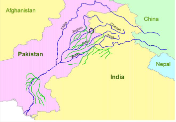
The Marala Ravi Link Canal off takes from River Chenab at Marala barrage, situated about 23 km towards the north-east of Sialkot city and 16 km from the foothills of Pir Punjal range, where Chenab River enters the plains near Akhnoor. The discharge of the river is influenced by two major tributaries (the Manawar Tawi and Jammu Tawi). Jammu Tawi is a flashy stream which brings a large amount of sediments and unfortunately, joins the river on the same side from which the canal off-takes. The capacity of the weir is

IJSER © 2014 http://www.ijser.org

International Journal of Scientific & Engineering Research, Volume 5, Issue 3, March-2014 3

ISSN 2229-5518

19800m3/s with an upstream pond level of 246.28 m. The location map of barrage is shown in Fig. 3. The heavy floods in the Monsoon season brings a large amount of sediments into the river due to erosion from the hilly
catchment area. These heavily sediment laden flow is diverted into the MRLC, consequently causes the aggradation of canal bed. The MRLC is a non–prenial and operates from 15th April to 15th October.
Designed May 2010 June 2010 July 2011 Aug 2011
243.500
243.000
242.500
242.000
241.500
241.000
240.500
152.4 228.7 304.9 609.8 914.6 1219.5 1524.4 1829.3 2134.1

Distance Along the Channel (m)

Fig.1 Bed level changes during 2010 and 2011

Fig. 2(a) Pictorial view of Sediment Deposition in MRL

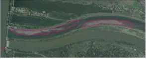
Fig. 2(b) Pictorial view of Sediment Deposition in

MRL

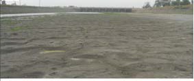
Fig. 2(c) Pictorial view of Sediment Deposition in

MRL

IJSER © 2014 http://www.ijser.org

International Journal of Scientific & Engineering Research, Volume 5, Issue 3, March-2014 4

ISSN 2229-5518

Fig 3(b) Map of study area

3 DATA COLLECTION AND ANALYSIS

Flows and sediment concentration is recorded at an interval
of six hours and twelve hours, respectively during the normal flow period. Flow is taken from the gauge reading in the canal whereas the sediment samples are collected from the each bay of canal. It is the responsibility of the staff of irrigation department to calculate the sediment concentration daily in the canal. They take the samples by inserting a steel sampler into the canal. The samples are then taken to the laboratory situated at the barrage location where they measure the sediment concentration. Bed profile is made from the sounding data at different cross-sections of the canal. The authors worked with the irrigation staff regularly for a period of two years (2011-2012) and collected the latest data in collaboration with the department. The previous record was taken from the irrigation department Sialkot and the Marala Barrage Division, the responsible authorities to collect and record the data.
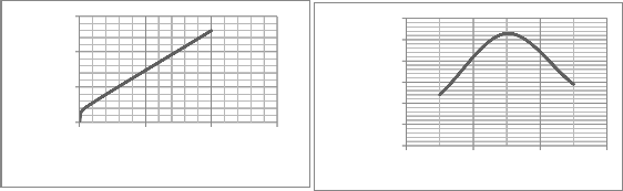
SSIIM requires input data for sediment sizes, fall velocities, roughness parameter, sediment parameters, and sediment concentrations which was estimated from the real data collected during the study period. The relation between sediment sizes and the fall velocity is shown graphically in Fig.4a. Fall velocity is directly proportional to the sediment sizes. As the size of the particle increases, velocity due to gravity increases. Different sediment sizes have different contribution in the total deposition in the canal. Fig. 4b shows the concentration of different sediment sizes in the flows. Silt particles (0.02 mm) have maximum concentration as compared to sand (0.13mm) and caly (0.002mm). The simulations by SSIIM for the sediment deposition were carried out for real flow conditions, fixed water surface, and
mobile bed conditions. The data collected during 2011 has been used for calibration of the model results. The time step of 120 seconds was used.

4 MATERIALS AND METHODS

The flow and sediment transport was carried out by using
Computaional Fluid Dynamics Model (CFD). SSIIM solves Reynolds Averaged Navier–Stokes (RANS) three dimensional equations to compute the water flows by the finite-volume descritazation method (Pederson 2012). The whole flow volume is divided into a mesh having very small dimensions in x, y and z directions. However high care is required to prepare grids and its control file. The convergence depends on proper development of grid and selection of suitable sediment and water flow parameters. The actual width of the canal (i.e. 110 m) and its actual geometry as trapezoidal channel was considered in the model. The whole width of the canal was divided into 15 parts. In this way the mesh size was taken as 7.33 m and
25m in x and y directions, respectively. Equally spaced eight layers were considered in z direction. The actual maximum water depth is 3.5 m in the canal at a design discharge of
623 cumecs. The length of the canal is selected in this study is 2.13 km because in this range most of the sediments are deposited and the behavior of the sediment concentration is well depicted for the installation of silt ejector.
The irrigation canals supply water according to the demand of the command area, therefore the flows varies in the canals according to the demand during different months. For this study, canal discharges ranging from 280 cumecs to 566 cumecs have been taken.

IJSER © 2014 http://www.ijser.org

International Journal of Scientific & Engineering Research, Volume 5, Issue 3, March-2014

5

ISSN 2229-5518

0.15
0.1
0.05
0
0 0.005 0.01 0.015
Sediment Sizes (mm)
0.0006
0.0005
0.0004
0.0003
0.0002
0.0001
0
0.13 0.02 0.002
Sediment Sizes (mm)
Fig. 4a Sediment size relationship with Fig4b Sediment size relationhip with
Fall Velocity Sediment Concentration
Sediment transport was computed using convection-diffusion equation, applying the van Rijin’s (1984a) formula with multiple grain sizes. Van Rijin’s equation (Olsen 2009,
2001) for Sediment concentration given in Eq. (1).

τ−τc 1.5

R = u∗d (6)

υ

where u* is the shear velocity, “d” is the particle’s diameter
and “υ” is the viscosity of water.
Velocity “U” for logarithmic profile is calculated by

C = X D 50

a 1 X

[ ]

τc

(ρs−ρw )g 1�

(1)

0.3

equation (7)

2 {D50 [

ρ υ2 ] 3 }

U 1
= ln �
30y

� (7)

where “Ca is the suspended sediment concentration,”
X1”and “X2” are the parameters, D50 is the sediment
particle diameter, ρS is the density of sediments taken as
2650 kg/m3, ρW is the density of water (i.e.1000kg/m3),υ is the kinematic viscosity of water (10-6 m2/s) and g is the gravitational acceleration (9.81 N/m2), τ is the shear stress and τc is the critical bed shear stress determined by the following equation (2)
u∗ k ks
where “u*” is the shear velocity, “k” is constant=0.4, “y” is
the flow depth and “ks” is the bed roughness height calculated by equation (8)
ks = (26 ∗ n)6 (8)
“u*” in equation 7 is calculated by equation (9)

τ

τ = ρwgyIf (2)
where ρw is the density of water, “y” is the depth of flow “g”
is the gravitational acceleration and “If” is the frictional slope. If is calculated as follows (equation (3))

u∗ = �

ρw

Hunter Rouse concentration “Cy”is calculated as
(9)


2 C y − h

= (
a

)z (10)

If = M2 y4/3 (3)

Ca h
y − a
where “M” is the Stickler’s coefficient “I” is the longitudanal
slope of the canal and “U” is the velocity which is calculated by equation (4)
where “y” is the water depth, “h” is the depth of each layer
from the bottom and the suspension parameter “z” is
calculated by equation (11)

2 1

U = Mr3 I2 (4)

w
z =
ku∗
(11)
“rh” is the hydraulic depth which is assumed to be equal to
the depth of flow because the width of the cross-section of the canal is very large. Critial shear stress is calculated by equation (5)

τc = Cg(ρs − ρw)D50 (5)

where τc is the critical shear stress, “C” is the Shield’s
parameter determined by Shield’s curve in which Reynolds
number is along abscissa and “C” is in ordinate. Reynolds number is calculated by equation (6)
where “w ” is the fall velocity and “kk” is constant = 0.4
Cell height is the height of each cell and cell flux is
calculated by multiplying the velocity, Hunter Rouse concentration and cell height. Hunter Rouse formula (eq.10) was used to compute the concentration in the center of each cell/layer, and the logarithmic velocity profile to compute the velocities (eq. 7). This can then be multiplied with the height of each cell to give an estimate of the suspended load. Table
1 describes the calculation of cell flux in vertical direction of flow at different depths.

IJSER © 2014 http://www.ijser.org

International Journal of Scientific & Engineering Research, Volume 5, Issue 3, March-2014 6

ISSN 2229-5518

Table 1: Calculated values of various sediment and flow parameters

5 RESULTS AND DISCUSSIONS

Calibration and validation is required for the analysis of any
real life problem for numerical models. In present study the model is calibrated by minimizing the error between the observed and the simulated values of water and bed levels. Bed roughness is an important parameter used in 3D modeling. So different values of roughness are optimized to check the most suitable value at which observed and simulated values of water and bed levels are close to each other. Model was calibrated and validated by setting the values of Manning’s constant “n” for bed roughness “ks” in k-ε model which gives minimum error between observed and simulated results. The values of Manning’s “n” used in optimization and sensitivity analysis were 0.0143, 0.017,
0.02 and 0.025.
The second important parameter is related to the sediment coefficients used in sediment load formula. Different trials were carried out to optimize the suitable value of sediment parameter X1 and X2 of equation 1. MATLAB was used for optimization of X1 and X2. Cell flux was compared with the observed values for all the layers and sum of square root error “E” was calculated by the eq. 12

1 n Cs(i) − Co(i) 2
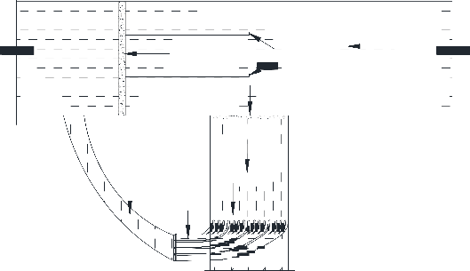
layers of the canal through tunnels spanning the whole width of the canal and discharges it into some nearby drain or back to river. Details of silt ejector are shown in Fig. 5a and 5b). It consists of a horizontal slab a little above the canal bed, which separates out the bottom layers. Under the slab there are tunnels to eject heavy silt laden bottom layers of water in an escape channel. The most important design parameters of silt ejector are its location and number of layers to be diverted back to the river.
The flow through the canal head regulator creates a lot of turbulence in the flow and throws a lot of sediment in suspension. This sediment starts settling down after a certain distance. The ejector is located close to the point where the sediment starts settling down and a fully developed flow is achieved. In this study the location was estimated by field visits.
To determine the height of perforated slab the impact of blocking one, two or three bottom layers was evaluated using simulations by SSIIM. Bed level changes after blocking one, two and three layers were simulated. As explained earlier, 8 layers of both water and sediments were defined in the control file. The width of canal was divided

E = �
n

� �

i=1

Cs(i) �
(12)
into 15 parts. To calculate the discharge through the ejector,
we have to calculate the discharge through each cell in the
Where Cs (i) is the simulated values and Co (i) is the
observed values of ith layer , “n” represents the number of
layers. The values of 0.015, 0.3 and 1.5 for X1 and 5%, 10%
geometry of the canal from intake to the ejector. The discharge for each layer through the ejector was calculated as under:

i i i i

15% and 20% of depth of flow for “X2” were used for
optimization process as explained by Olsen (2011). Optimization was done for each month (from May 2011 to October 2011). The data of April 2011 was taken as initial conditions. Remaining two months (Aug. and Sep. 2011)

Qs(i) = q1 + q2 + q3 +-------------+q15 13 where Qs(i)Qs is discharge passing through ith layer with

respect to eight layers in vertical direction. For the
calculation of discharge through silt ejector the following equation will be used in which i will vary from 1 to 3.
were selected for the validation process.
Qse = ∑3

Qs(i)

Silt ejector is the hydraulic structure located in the canal headreach such that sediment can be preiodically flushed back into the river. It remove the water from the bottom

i=1 14

where Qse “ Q is the total discharge in three bottom layers
passing through the silt ejector.

IJSER © 2014 http://www.ijser.org

International Journal of Scientific & Engineering Research, Volume 5, Issue 3, March-2014 7

ISSN 2229-5518

Regarding the silt ejector the results of simulations by SSIIM have shown that blockage of three layers with the help of silt ejector produces non silting non scouring situation. Hence the height of perforated slab of silt ejector was estimated to be 1.45 m (depth of each layer is 0.488 m and depth of 3 layers is 1.45m). The second design parameter as explained in the previous sections is the location of the silt ejector. It was estimated from the field

observations that the installing position of the ejector should be at the distance in between 140 to 150 m from the head regulator of the canal. The turbulent behavior of flow becomes dissipated after this distance and a fully developed flow was observed to be established.

Barrage

Divide Wall

River Flow

Head Regulator

MRL Canal

Silt Ejector

Escape

Diaphram

Tunnels

Clear Water

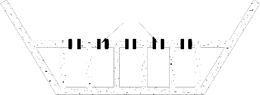
Fig. 5(a) Diagram of a silt ejector in canal

SLITS

Fig. 5 (b) Cross-section of tunnels

Fig. 5(a and b) Diagram of a silt ejector and the cross-section of the tunnel

6 CALIBRATION AND VALIDATION

Results of sensitivity analysis for both the roughness and
sediment parameters are shown in Fig. 6(a, b, c), Fig. 7 and Fig.8. The optimized value of “n” resulted to be 0.02 having minimum error in sediment concentration, bed levels and the water levels. So the optimized bed
roughness is 0.0197, calculated from equation 8. The optimized value of “X1” was obtained as 0.015 and “X2” was 15% of depth of flow.

IJSER © 2014 http://www.ijser.org

International Journal of Scientific & Engineering Research, Volume 5, Issue 3, March-2014 8

ISSN 2229-5518

The results of calibration and validation for bed level changes are shown in Fig.9. Simulated and observed water
0.12
0.1
0.08
0.06
0.04
0.02
0
0.0143 0.017 0.02 0.025
Manning's "n"
levels were also compared as shown in Fig. 10.
0.12
0.1
0.08
0.06
0.04
0.02
0
0.025 0.02 0.0167 0.0143
Manning's "n"
Fig. 6a Relationship b/w manning’s “n” Fig. 6b Relationship b/w manning’s “n”
and root mean square error in bed levels and root mean square error in sediment concentration
0.0061
0.0041
0.0021
0.0001
0.014 0.017 0.02 0.0215 0.03
Manning's "n"

Fig.6c Relationship b/w manning’s “n” and root mean square error of water levels
120
100
80
60
40
20
0
-20
1.5 0.015 0.3
Parameter X1

0.2

0.1

0

0.05y 0.10y 0.15y 0.20y

Parameter X2

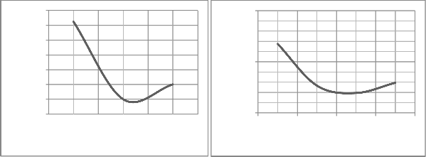
Fig. 7 Relationship b/w parameter “X1” Fig. 8 Relationship b/w parameter “X2” and root mean square error of sediment and root mean square error of sediment concentration concentration

IJSER © 2014 http://www.ijser.org

International Journal of Scientific & Engineering Research, Volume 5, Issue 3, March-2014 9

ISSN 2229-5518

243
241.5
240
152.44 228.66 304.88 609.76 914.63 1219.51 1524.39 1829.27 2134.15
Distance along the channel (m)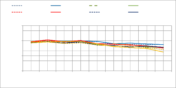

Fig. 9 Comparison b/w Observed bed levels and Simulated bed levels (May-Sep 2011)

Obs.(Sep) Simulated (Sep)
247
246.5
246
245.5
245
244.5
244
243.5
243
242.5
0 76.22 152.44 228.66 304.88 609.76 914.63 1219.51 1524.39 1829.27 2134.15
Distance along the channel (m)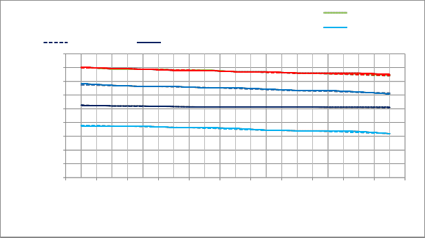

Fig. 10 Comparison b/w Observed Water levels and Simulate Water levels

7 General Simulation by SSIIM

The simulations have shown that small variations in roughness will strongly affect the bed formation pattern. Horizontal velocity decreases from top to bottom of the cross-section as shown in Fig. 11, while sediment

concentration has high values at the bottom where velocity is low. Further the sediment concentration is higher near banks than that the centre of the cross-section. Shear stress is also directly proportional to the turbulent

IJSER © 2014 http://www.ijser.org

International Journal of Scientific & Engineering Research, Volume 5, Issue 3, March-2014 10

ISSN 2229-5518

kinetic energy “K”. This is the reason due to which the sediment concentration is high in the bottom layers and at boundaries of the canal. The relation between velocities, “kinetic energy K” and shear stress is shown in table 2. Grids of the canal is shown in Fig. 11(a) and closed view

of highlighted portion of Fig. 11(a) is shown in 11 Fig.(b). Cross-section of the canal shows that bottom layers of the canal has less velocity as shown by the velocity vectors in Fig. 11(c).

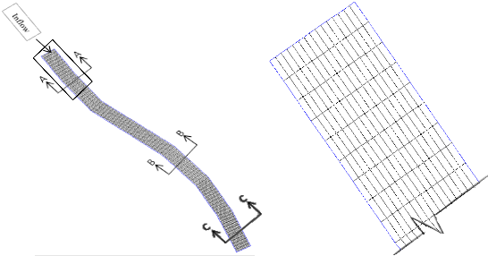
Fig. 11(a) Grids of MRL Canal Fig. 11(b) Closed view Grids of MRL Canal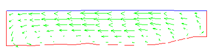

Fig.11(c) X-sections of the canal, less velocity at bottom layers and high in top layers
Velocity distribution and sediment concentration along the cross-section are shown below in Fig. 12 to Fig.17.

Left Bank Centre
Right Bank
Fig. 12 Velocity Distribution Section A-A

Left Bank Centre
Right Bank
Fig. 13 Sediment Concentration Section A-A

Left Bank Centre Right Bank
Fig. 14 Velocity Distribution Section B-B

IJSER © 2014 http://www.ijser.org

International Journal of Scientific & Engineering Research, Volume 5, Issue 3, March-2014

11

ISSN 2229-5518

Left Bank Centre
Right Bank

Fig. 15 Sediment Concentration Section B-B

Left Bank Centre Right Bank

Fig. 16 Velocity Distribution Section C-C

Left Bank Centre Right Bank

Fig. 17 Sediment Concentration Section C-C

Table 2 Relation b/w velocity, shear stress and “K” values

8 SUMMARY AND CONCLUSIONS

Sediment transport in MR Link canal in Pakistan has been investigated using field data and SSIIM model. It is concluded that the canal is suffering from the problem of deposition of silt in present conditions. This research has elaborated the usefulness of computational fluid dynamics model SSIIM for simulation of three- dimensional water flow coupled with sediment transport.

The most important elements of computational fluid dynamics modeling for sediment laden water in canals are the calibration coefficients, i.e. the equivalent roughness height and the sediment parameters. The Manning’s constant n was found to be 0.020. The optimized values of parameter “X1” and “X2” in Van Rijin’s sediment load formula are 0.015 and 15% of the

IJSER © 2014 http://www.ijser.org

International Journal of Scientific & Engineering Research, Volume 5, Issue 3, March-2014 12

ISSN 2229-5518

depth of flow of water in MR Link canal. Sediment deposition is more near to the banks of the channel because shear stress is more and velocity is less in that region.

A silt ejector should be installed in MR Link canal to

reduce the sediment deposition at the bed of channel so

that the efficiency of the canal is increased. The ejector should be placed at 140 to 150m from the intake and its perforated slab should be at a depth of 1.46m. The discharge through the ejector should be 46m3/s.

References:

[1] Agrawal AK (2005), Numerical modeling of sediment flow in Tala de-silting chamber, Master’s thesis Trondheim, Department of hydraulic and environmental engineering the Norwegian University of science and technology, D1-2005-12.

[2] Almerindo D. Ferreira, Sérgio R. Pinheiro, Sara C.

Francisco (2013), “Experimental and numerical study on the shear velocity distribution along one or two dunes in tandem”, Environmental Fluid Mechanics, volume 13, Issue 6, pp 557-570

[3] Arvandi S, Khosrojerdi, Rostami M and Baser H (2013) Simulation of interaction of side weir

overflows with bed-load transport and bed morphology in a channel (SSIIM 2), International Journal of water resources and environmental engineering, 5(5), 255-261,DOI

10.5897/IJWREE12.124

[4] Baranya S, Olsen NBR, Stoesser T, Sturm T (2013) A nested grid based computational fluid dynamics model to predict bridge pier scour, WaterManagement, DOI:10.1680/wama.12.00104

[5] Chohan MA (1986) Re-modeling Marala barrage

and link for silt control. In Proceedings of Pakistan engineering congress Lahore, Pakistan Paper No.

484

[6] Dissanayake K (2009) Experimental and numerical

modeling of flow and sediment characteristics in

open channel junctions, PhD thesis, School of civil

mining and environmental engineering University of Wollongong.

[7] Dong, N. H., Fang, C. M., and Cao, W. H. (2010). “Non-equilibrium sediment transport in the Three Gorges reservoir.” Journal of Hydraulics

Engineering. Vol. 41(6), 653–658 (in Chinese).

[8] Eilersten R, Olsen NBR, Ruther N, Zinke P (2013)

Channel bed changes in distributaries of the lake

Oyeren delta, southern Norway, revealed by

interferomatic side-scan sonar, Norwegian Journal

of geology, Vol 93,no. 1

[9] E. Dietze, F. Maussion, M. Ahlborn, B. Diekmann,

K. Hartmann, K. Henkel, T. Kasper, G. Lockot,

S. Opitz, and T. Haberzettl (2014), “Climate of the

past” doi:10.5194/cp-10-91-2014

[10] Elhakeem M., Krallis G., Prakash S., Edinger J.,

2008, Sediment Transport Modeling Review— Current and Future Developments, Journal of Hydraulics Engineering, Vol. 134, 1–14

[11] Ghumman AR, Khan RA, Khan QUZ, Khan Z (2012) Modeling for various design options of a canal

system, Water Resource Management, DOI

10.1007/s11269-012-0022-4

[12] Haun S (2011) Numerical modeling of flow over

trapezoidal broad-crested weir. Engineering

applications of computational fluid mechanics 5(3):

397-403.

[13] Haun, S, & Olsen, N (2012). Three-dimensional numerical modeling of the flushing process of the Kali Gandaki hydropower reservoir. Lakes & Reservoirs Research and Management 17, 25-33.

[14] Hoven L E (2010) Three-dimensional numerical

modeling of sediments in water reservoirs, Master’s thesis, Norwegian University of science and technology Faculty of Engineering science and technology department of hydraulic and environmental engineering.

[15] Huan S, Kjaeras H, Lovfall S, Olsen NBR (2013) Three dimensional measurements and numerical modeling of suspended sediments in a hydropower reservoir, Journal of hydrology vol 479,180-188

[16] Hussain M, Shakir A.S., Khan N.M., “Steady and

Unsteady Simulation of Lower Bari Doab Canal

using SIC Model”, Pak. J. Engg. & Appl. Sci. Vol. 12, pp 60-72.

[17] Irrigation Research Institute (1988) Marala Barrage—controlling silt entry into MR link: hydraulic model studies. Technical Report No. IRR-

902/Hyd/MR link, Lahore, Pakistan

[18] Jaan Hui Pu, Siow Yong Lim (2014), Efficient

numerical computation and experimental study of

temporally long equilibrium scour development

around abutment,” Environmental fluid

mechanics” , Volume 14, Issue 1, pp 69-86

[19] Jia D. D., Shao X. J. Zhang X. N., and Ye Y. T.,

(2013), Sedimentation Patterns of Fine-Grained

Particles in the Dam Area of the Three Gorges

IJSER © 2014 http://www.ijser.org

International Journal of Scientific & Engineering Research, Volume 5, Issue 3, March-2014 13

ISSN 2229-5518

Project: 3D Numerical Simulation, Journal of

Hydraulics Engineering ,Vol. 139(6):669-674.

[20] Jia, D. D., Shao, X. J.,Wang, H., and Zhou, G. (2010).

Three-dimensional modeling of bank erosion and morphological changes in the Shishou bend of the middle Yangtze River. Adv. Water Resource, 33(3),

348–360

[21] Jia, D. D., Shao, X. J.,Wang, H., and Zhou, G. (2010).

“Three-dimensional modeling of bank erosion and morphological changes in the Shishou bend of the middle Yangtze River.” Adv. Water Resource, 33(3),

348–360

[22] Lu, Y. J., and Wang, Z. Y. (2009). “3D numerical

simulation for water flows and sediment deposition in dam areas of the three gorges project.” Journal of Hydraulics Engineering, Vol. 135(9), 755–769.

[23] Munir S, Schultz B, Suryadi F.X, Hoanh C T (2009) Managing sedimentation in downstream control Irrigation canals. 60th International Executive

council meeting 7 5th Asian regional conference, 6-

11 December 2009, New Dehli, India.

[24] Olsen NBR (2001) CFD modeling for hydraulic

structures by, preliminary 1st edition, ISBN 82-7598-

048-8

[25] Olsen NBR (2007) Numerical Modeling and Hydraulics. Class notes, Department of Hydraulic and Environmental Engineering the Norwegian University of science and technology, 1st edition, 10

September 2007 ISBN 82-7598-074-7.

[26] Olsen NBR (2009) Numerical modeling and hydraulics. Department of Hydraulic and Environmental Engineering the Norwegian University of science and technology, 3rd edition, ISBN 82-7598-074-7.

[27] Olsen NBR (2011). A Three-dimensional numerical

model for simulation of sediment movements in water intakes with multi-block option. User’s manual, Department of hydraulic and environmental engineering the Norwegian University of science and technology.

[28] Pedersen O (2012) 3D numerical modeling of hydro- speaking scenarios in Norwegian regulated rivers. Master’s thesis, Department of Hydraulic and Environmental Engineering the Norwegian University of science and technology

[29] Punjab irrigation department (1994), Detailed engineering designs for restoration and improvement of MR link canal system. PC II

[30] Punjab Irrigation Department (PID) Departmental records and files on MRL canal system and Marala

Barrage. Lahore, Pakistan

[31] Ruether N (2006) Computational fluid dynamics in fluvial sedimentation engineering, PhD thesis, The Norwegian University of science and technology.

[32] Ruether N, Singh JM, Olsen NBR, Atkinson E (2005)

3D computation of sediment transport at water

intakes, Water Management 158, paper no.13849:1–8

[33] S. N. Chan, Ken W. Y. Lee, Joseph H. W. Lee

(2014), Sediment-laden turbulent flows are

commonly encountered in natural and engineered environments, Environmental fluid mechanics, vol

14 issue 1 pp 173-200

[34] Shakir AS, Haq AU (1999) Remodeling approach for

large canals: a case study of Marala Ravi link canal

Pakistan. In: Proceedings of 17th congress of international commission on irrigation and drainage (ICID), Granada, Spain

[35] Shakir AS, Haq AU, Shahid BA (1996) Restoring design capacity of Marala Ravi Link canal. In Proceedings of 66th annual session of Pakistan

engineering congress, Lahore, Pakistan. Paper no.

556

[36] Tommaso Lucchini, Marco Fiocco, Roberto torelli,

Gianluca D’Errico (2014), Automatic Mesh

Generation for Full-Cycle CFD Modeling of IC

Engines”, “SAE international”, 2014-01-1131

[37] Van Rijn, L.C., 1984a. Sediment transport, Part II:

suspended load transport. Journal of Hydraulic

Engineering, ASCE 110 (11), 1613–1641.

[38] Zhang Q, Hillebrand g, klassen I, Vollmer S, Olsen

NBR, Moser H and Hinkelmann R (2013) Sensitivity analysis of floe field simulation in the Iffezheim reservoir in Germany using the 3D SSIIM model, IAHR 35th congress, Chengdu, China

IJSER © 2014 http://www.ijser.org