International Journal of Scientific & Engineering Research, Volume 5, Issue 7, July-2014 723

ISSN 2229-5518

Security Constrained Unit Commitment Based Load and Price Forecasting Using Evolutionary Optimized LSVR

Ehab E. Elattar, Member, IEEE, and Tamer A. Farrag

Abstract— In this paper, a local predictor approach based on proven powerful regression algorithm which is support vector regression (SVR) combined with space reconstruction of time series is introduced. In addition, real value genetic algorithm (GA) has been utilized in the proposed method for optimization of the parameters of the SVR. In the proposed approach, the embedding dimension and the time delay constant for the load and price data are computed firstly, and then the continuous load and price data are used for the phase space reconstruction. Subsequently, the reconstructed data matrix is subject to the local prediction algorithm. Then the forecasted loads and price are fed into IEEE 30 bus test system for security constraint unit commitment to show the reactions of unit commitment to load and price forecasting errors. The proposed model is evaluated using real world dataset. The results show that the proposed method provides a much better performance in comparison with other models employing the same data.

Index Terms— Load forecasting, price forecasting, local predictors, security constrained unit commitment, support vector regression, genetic algorithm, state space reconstruction.

——————————  ——————————

1 INTRODUCTION

HORT term load forecasting (STLF) is a vital part of the op- eration of power systems. STLF aims to predict electric loads for

a period of minutes, hours, days, or weeks. STLF has always been a very important issue in economic and reliable power systems opera- tion such as unit commitment, reducing spinning reserve, mainte- nance scheduling, etc.
Several STLF methods including traditional and artificial
intelligence-based methods have been proposed during the
last four decades. The relationship between electric load and
its exogenous factors is complex and nonlinear, making it quite difficult to be modeled through traditional techniques such as linear or multiple regression [1], autoregressive mov- ing average (ARMA), exponential smoothing methods [2],
Kalman-filter-based methods [3], etc. On the other hand, vari- ous artificial intelligence techniques were used for STLF; among these methods, artificial neural networks (ANNs) have received the largest share of attention. The ANNs that have been successfully used for STLF are based on multilayered perceptrons [4]. The neural fuzzy network has also been used for load forecasting [5]. Radial basis functions (RBFs) [6] have been also used for day-ahead load forecasting, giving better results than that of the conventional neural networks.
Accurate forecasting of the electricity price has become a

————————————————

• This work was supported byTaif University, KSA under grant 3267-435-1.

• The Authors are with the department of the Electrical Engineering, Faculty of Engineering, Taif University, Kigdom of Saudi Arabia.

• Ehab E. Elattar on leave from the Department of Electrical Engineering, Faculty of Engineering, Menofia University, Shebin El-Kom, Egypt

(e-mail: dr.elattar10@yahoo.com).

• Tamer A. Farrag is on leave from the Department of Communications and

Electronics, Misr high institute of Engineering and Technology, Egypt.

very valuable tool. This is because of the upheaval of deregu- lation in electricity market. Short-term price forecasting in a competitive electricity market is still a challenging task be- cause of the special electric price characteristics [7], [8], such as high-frequency, non-stationary behavior, multiple seasonality, calendar effect, high volatility, high percentage of unusual prices, hard non-linear behavior etc.
In the literature, several techniques for short-term electrici-
ty prices forecasting have been reported, namely traditional
and AI-based techniques. The traditional techniques include
autoregressive integrated moving average (ARIMA) [9], wave-
let-ARIMA [10] and mixed model [11] approaches. Although, these techniques are well established to have good perfor-
mance, they cannot always represent the non-linear character- istics of the complex price signal. Moreover, they require a lot of information, and the computational cost is very high.
On the other hand, AI-based techniques have been used by many researchers for the price forecasting in electricity mar- kets. These methods can deal with the non-linear relation be- tween the influencing factors and the price signal, therefore the forecasting precision is raised. These techniques include neural network (NN) [12], radial basis function NN [13], fuzzy neural network (FNN) [14] and hybrid intelligent system (HIS) [15]
Recently, SVR [16], [17] has also been applied successfully
to STLF and price forecasting. SVR replaces the empirical risk
minimization which is generally employed in the classical
methods such as ANNs, with a more advantageous structural
risk minimization principle. SVR has been shown to be very
resistant to the over fitting problem and give a high generali- zation performance in forecasting problems [18].
All the above techniques are known as global predictors in which a predictor is trained using all data available but give a prediction using a current data window. The global predictors suffer from some drawbacks which are discussed in our pre- vious work [19], [20]. To overcome these drawbacks, the local

IJSER © 2014 http://www.ijser.org

International Journal of Scientific & Engineering Research, Volume 5, Issue 7, July-2014 724

ISSN 2229-5518

SVR predictor is proposed in our previous work [19]–[21] and can be used to solve the STLF and price forecasting problem.
Phase space reconstruction is an important step in local prediction methods. The traditional time series reconstruction techniques usually use the coordinate delay (CD) method [22] to calculate the embedding dimension and the time delay con- stant of the time series [23].
Although local SVR (LSVR) method gives good prediction accuracy when it is applied to STLF and price forecasting, it has a serious problem. This problem is that there is a lacking of the structural methods for confirming the selection of SVR’s parameters efficiently. So, in this paper, a local predictor ap- proach based on proven powerful regression algorithm which is SVR combined with space reconstruction of time series is introduced. In addition, real value genetic algorithm (GA) has been utilized in the proposed method for optimization of the parameters of the SVR. The proposed algorithm is called evo- lutionary optimized LSVR (EOLSVR).
Unit commitment problem (UC) is a nonlinear, mixed in- teger combinatorial optimization problem. The UC problem is the problem of deciding which electricity generation units should be scheduled economically in a power system in order to meet the requirements of load and spinning reserve. It is a difficult problem to solve in which the solution procedures involve the economic dispatch problem as a sub-problem. Since UC searches for an optimum schedule of generating units based on load forecasting data, the improvement of load forecasting is first step to enhance the UC solution [24].
In this paper, we propose security constrained unit com- mitment (SCUC) method to reduce the production cost by combining load and price forecasting with UC problem. First, short-term loads and price are forecasted using EOLSVR, local SVR and local RBF models. Then UC problem is solved using the dynamic programming method.
We have chosen the historical data for the South Australia electricity market, which includes the power demand and price for the period of 2003-2005. Historical weather data was collected from Macquarie University Web Site. Then the fore- casted loads and price are fed into IEEE 30 bus test system for unit commitment to show the reactions of unit commitment to forecasting errors.
The paper is organized as follows: Section 2 review the time series reconstruction method. Section 3 gives a brief dis- cribtion about GA. A review of the SCUC problem and its formulation are presented briefly in Section 4. The proposed method is presented in details in Section 5. Applications and simulations for load and price forecasting and UC problem are given in Sections 6. Finally, Section 7 concludes the work.

2 TIME SERIES RECONSTRUCTION

Nonlinear time series analysis and prediction have be- come a reliable tool for the study of complex time series and dynamical systems. A commonly used tool is the phase space reconstruction technique which stems from the embedding theorem developed by Takens and Sauer [22], [25]. It illus- trates clearly the phase space trajectory of a time series in the
embedded space instead of the trajectory in the time domain. The theorem regards an 1-dimensional time series x(t) for t =

1, 2, ...,N as compressed higher dimensional information and, thus, its features can be extracted by extending x(t) to a vector X(t) in a d-dimensional space as follows:

X (t ) = [x(t ), x(t − m), x(t − 2m),...., x(t − (d − 1)m)] (1)

where d denotes the embedding dimension of the system and m is the delay constant. Based on Takens’ theorem [22], to obtain a faithful reconstruction of the dynamic system, the embedding dimension must satisfy d2 ≥ Da +1, where Da is the dimension of the attractor. In order to obtain an appropriate model reconstruction, it is necessary to estimate d and m.

The correlation dimension method [26] is the most popu- lar method for determining d because of its computational simplicity. The mutual information method proposed in [27] usually provides a good criterion for the selection of m. In general, the proper value of m corresponds to the first local minimum of mutual information. In this paper, the correlation dimension method [26] and the mutual information method [27] are used to calculate d and m respectively. The details of how to choose the proper values of d and m using these two methods have been reported in [19].

3 GENETIC ALGORITHM

The GA is a search algorithm for optimization, based on the mechanics of natural selection and genetics [28], [29]. The GA is able to search very large solution spaces efficiently by providing a lower computational cost, since they use probabil- istic transition rules instead of deterministic ones. GA has a number of components or operators that must be specified in order to define a particular GA. The most important compo- nents are representation, fitness function, selection method, crossover, mutation and termination.
The GA starts with an initial population of individuals (generation) which are generated randomly. Every individual (chromosome) encodes a single possible solution to the prob- lem under consideration. The fittest individuals are selected by ranking them according to a pre-defined fitness function, which is evaluated for each member of this population. The individuals with high fitness values therefore represent better solution to the problem than individuals with lower fitness values.
There are many different selection operators presented by some researchers such as stochastic sampling with replace- ment”roulette wheel selection” and tournament selection [30]. Following this initial process, the crossover and mutation op- erations are used where the individuals in the current popula- tion produce the children (offspring). The idea behind the crossover operator is to combine useful segments of different parents to form an offspring that benefits from advantageous bit combinations of both parents [31]. While, by mutation, in- dividuals are randomly altered. These variations (mutation steps) are mostly small [31]. Normally, offspring are mutated after being created by crossover. It is intended to prevent

IJSER © 2014 http://www.ijser.org

International Journal of Scientific & Engineering Research, Volume 5, Issue 7, July-2014 725

ISSN 2229-5518

premature convergence and loss of genetic diversity. A new
population of individuals (generation) is then formed from the
where,

t

on,i

is the number of hours the unit has been on
individuals in current population and the children. This new population becomes the current population and the iterative cycle is repeated until a termination condition is reached [28].

4 SECURITY CONSTRAINT UNIT COMMITMENT (SCUC)

line and T up is the minimum up time.

Minimum down time: Once the unit is turned off, it is not allowed to be brought online again before spending certain number of hours called minimum down time. This can be formulated as follows:

The objective of security-constrained unit commitment
(SCUC) discussed in this work is to obtain a unit commitment

t −1

off ,i

− Ti

down

)(u t

− u t −1

)≥ 0

schedule at minimum production cost without compromising the system reliability. The reliability of the system is interpret- ed as satisfying two functions: adequacy and security. In sev-

t

off ,i

where t

t −1

off ,i

+ 1)(1 − u t )
(6)
eral power markets, the independent system operator ISO

X off ,i

line and down
is the number of hours the unit has been off

Ti is the minimum down time.

plans the day-ahead schedule using (SCUC)[32], [33].
The traditional unit commitment algorithm determines the unit schedules to minimize the operating costs and satisfy

Spinning reserve: It can be modeled as follows:

N

∑ u t P max ≥ Dt + Rt

(7)
the prevailing constraints such as load balance, system spin- ning reserve, ramp rate limits, fuel constraints, multiple emis- sion requirements and minimum up and down time limits
over a set of time periods. The scheduled units supply the load

i i i

where Rt is the spinning reserve requirements.

Transmission flow limit from bus k to bus m:

demands and possibly maintain transmission flows and bus

P max ≤ P

(t ) = f (P(t ), ϕ (t )) ≤ p max
(8)
voltages within their permissible limits [34]. However, in cir- cumstances where most of the committed units are located in one region of the system, it becomes more difficult to satisfy the network constraints throughout the system.
Mathematically, the objective function, or the total operat- ing cost of the system can be written as follows [32], [33]:

km km km

where P(t) is the real power generation vector and φ(t) is the phase shifter control vector at time T.
The Start up cost which can be modeled by the following form:

min ∑ ∑

ut [F (Pt )+ S t (1 − ut − 1)]

(2)

HS i ,

t = 

if X t

≤ T down + CH i

 T N

t 



i i i i i 



Si 

off , i i

Pi uit  t = 1i = 1 

 i

CS ,

if X t

> T down + CH i

(9)
where
Pt is the output power of unit i at period t, u t is

 off , i i

i

the commitment state of unit i at period t,

F (Pt ) is the fuel

i i where,

HS i , CS i is the unit’s hot/cold start up cost and

cost of unit i at output power Pt ,

S t is the start up price of

CH i is the cold start hour.

unit i at period t, N is the number of generating unit and T is
the total number of scheduling periods.

Fuel cost functions F (Pt )

is frequently represented by
The constraints are as follows:

Power balance:

the following polynomial function:

N

∑ u t Pt = Dt

(3)

F (Pt )= a

+ b Pt + c (Pt )2

(10)

i i i

i i i i i i i

where ai , bi , ci

are the coefficients for the quadratic cost
where Dt is the customers’ demand in time interval t.

Generating limits: These limits define the region within which a unit must be dispatched.

curve of generating unit i.

5 EVOLUTIONARY OPTIMIZED LOCAL SUPPORT VECTOR

t min

i i

≤ Pi

≤ u t P

max

(4)

REGRESSION (EOLSVR)

5.1 Support Vector Regression (SVR)

Minimum up time: Once the unit is committed, it must be

kept running for certain number of hours, called the minimum up time, before allowing turning it off. This can be formulated as follows:
The basic idea of SVR is to map the data x into a high di- mensional feature space via a nonlinear mapping, and per- form a linear regression in that feature space [17] as:

(X t −1

T up )(u t −1

u t )

f (x ) =

w, x + b

(11)

on,i − i

i − i ≥ 0

X t = (X t −1 + 1)u t

(5)

on,i

on,i i

IJSER © 2014 http://www.ijser.org

International Journal of Scientific & Engineering Research, Volume 5, Issue 7, July-2014 726

ISSN 2229-5518

Where 〈., .〉 denotes the dot product, w contains the coeffi- cients that have to be estimated from the data and b is a real constant. Using Vapink’s ε–insensitive loss function [16], the overall optimization is formulated as:
First, reconstruct the time series as described in the previ- ous section. For, each query vector q, the K nearest neighbors
{zq 1,zq 2,...,zq K} among the training inputs is choosing using the
Euclidian distance as the distance metric between the q and each z in the reconstructed time series. Using these Knearest

1 T N *

min w

w,b,ξ ,ξ * 2

w + C ∑ (ξi + ξi )

i=1

neighbors, train the SVR (or RBF) to obtainsupport vectors and
corresponding coefficients. Finally, the output of SVR (or RBF)

 y − (wT φ (x ) + b ) ≤ ε + ξ *

can be computed.

i i i

subject to (w φ (x ) + b ) − y

≤ ε + ξ

5.3 EOLSVR

 T i i i

 *

(12)
There are some key parameters for SVR, which are C, ε

ξi , ξi ≥ 0,

i = 1,..., N

and σ in the Gaussian kernel function. The selection of these parameters is important to the generalization of the predic-
where, xi is mapped to higher dimensional space by the

*

tion. Inappropriate parameters in SVR lead to overfitting or
function φ, ε is a real constant, ξi and ξi
are slack variables
under-fitting [35]. Therefore, these parameters must be chosen
subject to ε-insensitive zone and the constant C determines the
trade-off between the flatness of f and training errors.
Introducing Lagrange multipliers αi and αi * with αi αi *=0 and αi , αi *=0 for i=1,…,N, and according to the Karush-Kuhn- Tucker optimality conditions [17], the SVR training procedure amounts to solving the convex quadratic problem:
carefully. However choosing the optimal parameters is a very important step in SVR, there are no general guidelines availa- ble to select these parameters till now. The problem of optimal parameters selection is very complicated because the complex- ity of SVR (and hence its generalization performance) depends on all three parameters together. Thus, a separate selection of each parameter is not adequate to get an optimal regression

1 min

∑ (α

− α * )(α

− α * )Q(x , x )+

model.

α ,α * 2 i , j =1 i i j j i j

N N

ε ∑ (α i + α i )− ∑ yi (α i − α i )

There are many trials to choose the SVR’s parameters.
Various authors have selected these parameters by experience
[16], [36] but this method is not suitable for nonexpert users.

i=1

* *

i=1

The grid search optimization method has been proposed by

0 ≤ α i , α i ≤ C

Scholkopf and Smola [37] to get the optimal parameters of

subject to 

N ( * )

(13)
SVR. However, this method is time consuming. The cross val-

∑i=1 α i − α i

= 0, i = 1,..., N

idation method has been also used to select the SVR’s parame-
The output is a unique global optimized result that has the form:
ters [36]. This method is very computationally intensive and data-intensive. Pai and Hong proposed a GASVR model [38] to optimize the SVR’s parameters in which the parameters are

 N

f ( x) = ∑ (α

− α * )Q( x , x

) + b

(14)
encoded as a binary code. This method suffers from some

i i i j

i=1

where, Q(xi,x)= φ(xi). φ (x). Using kernels, all necessary computations can be calculated directly in the input space, without computing the explicit map φ(x). Various kernel types exist such as linear, hyperbolic tangent, Gaussian, polynomial, etc. [17]. Here, we employ the commonly used Gaussian ker- nel which can be as defined as following:
problems. The first one is that encoding the parameters as bi-
nary code will lead to integer valued solutions and may suffer from the lack of accuracy [29]. In addition, if the length of the string is not long enough, it might be possible for the GA to get near to the region of the global optimum but never will arrive at it.
As evident from above, there is a lacking of the structural methods for confirming the selection of SVR’s parameters effi-
ciently. Therefore, a real value GA is proposed in this work to



Q( x , x) = exp −

x − x 



(15)
select the SVR’s parameters of local SVR method which simul-

i

5.2 Local predictors

 2σ 2 

taneously optimizes all SVR’s parameters from the training data. The steps for load and price forecasting based on the proposed method can be summarized as following:
Local prediction is concerned with predicting the future
based only on a set of K nearest neighbors in the reconstructed embedded space without considering the historical instances which are distant and less relevant. Local prediction con- structs the true function by subdivision of the function domain into many subsets (neighborhoods). Therefore, the dynamics of time series can be captured step by step locally in the phase space and the drawbacks of global methods can be overcome.
• Step 1: Reconstruct the time series: Load the multivar ate
time series dataset X = (x1 (t), x2 (t), ..., xM (t)), (t =1, 2, ...,N). Using the correlation dimension method and the mutual information method, calculate the embedding dimension d and the time delay constant m for each time series data set. Then, reconstruct the multivariate time series using these values.
• Step 2: Form a training and validation data: The input da-
~
The local SVR (LSVR) and local RBF (LRBF) methods can
taset after reconstruction X
is divided into two parts, that
be summarized as follows [19]:

IJSER © 2014

is a training

~ dataset and validation

~ dataset. The

http://www.ijser.org

International Journal of Scientific & Engineering Research, Volume 5, Issue 7, July-2014 727

ISSN 2229-5518

size of the training dataset is Ntr while the size of the vali- dation dataset is Nva .
• Step 3: For each query point xq, choosing the K nearest
neighbors of this query point using the Euclidian distance
between xq and each point in Xtr (1 < K<<< ~ ).

X tr

• Step 4: Representation and generation of initial population:
In real value GA the real value parameters can be used di- rectly to form the chromosome. This means that the chro- mosome representation in real value GA is straightfor- ward. In this case, the three parameters C, ε and σ are di- rectly coded to generate the chromosome CH = {C, ε, σ}. These chromosomes are all randomly initialized.
• Step 5: Evaluation: each chromosome is evaluated using
the fitness function which measures the performance of the model. It is quite important for evolving systems to find a good fitness measurement. The fitness (F) of each chromo- some evaluated using mean absolute percentage error (MAPE) defined as:

6 EXPREMENT RESULTS

In this paper, the performance of the EOLSVR is tested and compared with local SVR and local RBF using hourly load price and temperature data in South Australia. The load data used includes hourly load and price for the period of 2003-
2005 for the South Australia electricity market. While the hourly temperature for the same period is collected from Macquarie university web site.

6.1 Parameters

To implement a good model, there are some important pa- rameters to choose. Choosing the proper values of d and m is a critical step in the algorithm. The correlation dimension meth- od and the mutual information method are used to select d and m, respectively, and the optimal values of these parame- ters are shown in Table 1. Using the obtained values of d and m, the multivariate time series can be reconstructed as de- scribed in Section 2.
MAPE =
1

N va

N va

∑

i =1

Ai − Fi

Ai

× 100
(16)
TABLE 1

PHAE RECONSTRUCTION PARAMETERS

where Ai and Fi are the actual value and the forecasted value, respectively, Nva is the validation dataset size, and i denotes the test instance index.
• Step 6: Selection: A standard roulette wheel selection method is employed to select the fittest chromosomes from the current population.
• Step 7: Crossover: The operator of crossover can now be
implemented to produce two offspring from two parents which are chosen using the roulette wheel selection meth- od. In this work, the line arithmetical crossover is used [28].
Choosing K is very important step in order to establish the local prediction model. There are some methods used in litera- tures to find this parameter. In this paper K is calculated using a systematic method which is proposed by us in [20]:
• Step 8: Mutation: Similarly, the mutation operation can

 α N

kmax

 (17)

contribute effectively to the diversity of the population. In

K = round 

N × k × D

∑ ∑ Dk ( xi ) 

this work, the Gaussian mutation [28] is used.

 max

max

i =1 k =1 

• Step 9: Elitist strategy: The chromosome that has the worst fitness value in the current generation is replaced by the chromosome that has the best fitness value in the old gen-

where, N is the number of training points, kmax is the max- imum number of nearest neighbors, Dk (xi) is the distance be-

tween each training point x and its nearest neighbors while

1 N kmax ( )

eration
• Step 10: Check the stopping criterion: The modelling can be

Dmax is the maximum distance,

N × k

max

× Dmax

∑i =1 ∑k =1 Dk xi

terminated when the stopping criterion is reached. In this work, we use a predetermined maximum number of gen- erations as a termination condition. If the stopping criteri- on is not satisfied, the model has to be expanded, the steps
5 to 9 can be repeated until the stopping criterion is satis- fied.
• Step 11: After the termination condition is satisfied, the
chromosome which gives the best performance in the last generation is selected as the optimal values of SVR’s pa- rameters.
• Step 12: Train SVR: The K nearest neighbors of the query
point and the optimized parameters are used to train the
SVR algorithm.
is the average distance around the points which is inversely
proportional to the local densities and α is a constant. The two constants kmax and α are very low sensitivity parameters. kmax
can be chosen as a percentage of the number of training points (N) for efficiency while α can be chosen as a percentage. In this paper, kmax and α are always fixed for all test cases at 70% of N and 95, respectively.

6.2 Forcasting Accuracy Evaluation

For all performed experiments, we quantified the predic- tion performance with the Mean Absolute Error (MAE) and Mean Absolute Percentage Error (MAPE). They can be defined as follows:

n

• Step 13: Calculate the prediction value of the current query point using equation (14).
• Step 14: Then, the steps 3 to 13 can be repeated until the

MAE = 1 ∑ A(i) − F (i)

n i =1

(18)
future values of different query points are all acquired.

IJSER © 2014

MAPE = 1 ∑

A(i) − F (i)

( )

×100

http://www.ijser.org

n i =1 A i

International Journal of Scientific & Engineering Research, Volume 5, Issue 7, July-2014 728

ISSN 2229-5518

(19)

S

where, A and F are the actual and the forecasted loads, re- spectively, n is the testing dataset size, and i denotes the test instance index.

6.3 Results and Discussion

The performance of the evolutionary optimized local SVR (EOLSVR) is tested and compared with local SVR and local RBF using hourly load, price and temperature data in South Australia.
To make results comparable, the same experimental setup is used for the three predictors. That is the week of February
15-21, 2005 has been used as a testing week. The available hourly load and temperature data (for the period of 2003-2005) are used to forecast the load of testing week. Also, the availa- ble hourly price and temperature data (for the period of 2003-
2005) are used to forecast the price of testing week.
First, we calculate the MAE and MAPE of each day during
the testing week. Then the average MAE and MAPE values of
each method for the testing week are calculated. The results
are shown in Tables 2 and 3.
These results show that, the EOLSVR method outperforms local SVR and local RBF. Table 4 shows the MAE improve- ments of the EOLSVR method over local SVR and local RBF. While Table 5 shows the MAPE improvements of the EOLSVR method over local SVR and local RBF. These results show the

TABLE 2

LOAD FORECASTING RESULTS

superiority of the proposed method over other methods.

TABLE 3

Price Forecasting Results

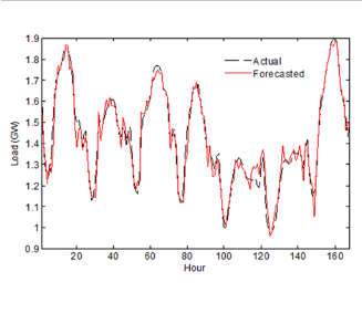
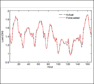
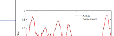
Figures 1-3 show the actual load and forecasted load val- ues using local RBF, local SVR and EOLSVR, respectively for the testing week.
TABLE 4

IMPROVEMENT OF THE EOLSVR OVER OTHER APPROACHES

REGARDING MAE

Fig. 2 Forecasted and actual hourly load from 15th to 21st February

2005 using local SVR

IJSER © 2 http://www.ijse

International Journal of Scientific & Engineering Research, Volume 5, Issue 7, July-2014 729

ISSN 2229-5518

The results of load and price forecasting are fed into the IEEE 30 bus test system. The IEEE 30 bus test system is used with a total of 6 generators and 41 lines. Table 6 shows the test system data. The spinning reserve is assumed to be 10% of the demand. The actual loads (24 hour) as well as the forecasted loads are given in Table 7.
If the initial commitment state of a generator is 1, it means this generator is on and zero indicates this generator is off. The IEEE 30 bus test system has 41 lines. Each line can transmit a maximum power flow in MW. Table 8 shows the maximum power flow for each line
Feasible unit combination and total cost (TC) values of the test system using dynamic programming method for load val- ues and forecasting load values are given in Table 9. It is clear that accurate load forecasting is very important for the UC solution. The total cost of the forecasting load values for local RBF method is more than that of actual load values by
$13140.6. Additionally, the total cost of the forecasting load values for local SVR is more than that of actual load values by
$5016. Whereas the total cost of the forecasting load values for
EOLSVR is more than that of actual load values by $3341.1.

7 CONCLUSION

In this paper, we have proposed EOLSVR method for elec- trical load and price forecasting. After that the results of load and price forecasting are used to solve the security constraint unit commitment problem.
The proposed method combines a proven powerful regres- sion algorithm which is SVR with a local prediction frame- work. For data preprocessing, the embedding dimension and the time delay constant for the input data are computed firstly, and then the continuous load and price data are used for the phase space reconstruction. In addition, the neighboring points are presented by Euclidian distance. According to these neighboring points, the local model is set up. The local predic- tors can overcome the drawbacks of the global predictors by involving more than one model to utilize the local infor- mation. Therefore, the accuracy of the local predictor is better
than the global predictor in which only one model is engaged for all available data that contains irrelevant patterns to the current prediction point. In addition, to set the SVR’s parame- ters appropriately, a new method is proposed. This method adopts real value GA to seek the optimal SVR’s parameters values and improves the prediction accuracy. Then the fore- casted loads and price are fed into IEEE 30 bus test system for security constraint unit commitment to show the reactions of unit commitment to load and price forecasting errors.
Dynamic programming method is used for solving the UC problem. Total costs are calculated for load data which is tak- en from South Australia electricity market and forecasting load and price data computed by local RBF, local SVR and EOLSVR, separately. Comparing these total costs show that accurate load forecasting is important for UC. Over-prediction of STLF wastes resources since more reserves are available than needed and, in turn, increases the operating cost. On the other hand, under-prediction of STLF leads to a failure to pro- vide the necessary reserves which is also related to high oper- ating cost due to the use of expensive peaking units.

ACKNOWLEDGMENT

The authors gratefully acknowledge the Taif University for its support to carryout this work. It funded this project with a fund number 3267-435-1.

REFERENCES

[1] A. D. Papalekopulos and T. C. Hesterberg, “A regression-based approach to short-term system load forecasting,” IEEE Trans. Power Syst., 5 (4), 1535–1547, Nov. 1990.

[2] J. W. Taylor, L. M. de Menezes, and P. E. McSharry, “A comparison of uni- variate methods for forecasting electricity demand up to a day ahead,” Int. J. Forecasting, 22 (1), 1–16, 2006.

[3] J. H. Park, Y. M. Park, and K. Y. Lee, “Composite modeling for adaptive short- term load forecasting,” IEEE Trans. Power Syst., 6 (2), 450–457, May 1991.

[4] H. S. Hippert, C. E. Pedreira, and R. C. Souza, “Neural networks for short term load forecasting: A review and evaluation,” IEEE Trans. Power Syst., 16 (1), pp. 44–55, Feb. 2001.

[5] C. J. Lin, C. H. Chen, and C. T. Lin, “A hybrid of cooperative particle swarm optimization and cultural algorithm for neural fuzzy networks and its predic- tion applications,” IEEE Trans. Syst.,Man, Cyber. C, Appl. Rev., 39 (1), 55–68, Jan. 2009.

[6] S. Sheng and C. Wang, “Integrating radial basis function neural network with fuzzy control for load forecasting in power system,” in Proc. IEEE Trans. Dist. Conf. Exhib. Asia and Pacific, 2005, pp. 1–5.

[7] C. Martos, J. Rodriguez, and M. Sanchez, ‘Forecasting electricity prices by extracting dynamic common factors: application to the Iberian Market’, IET Gener. Transm. Distrib., 6, (1), 11–20, 2012.

[8] L. Saini, S. Aggarwal, and A. Kumar, ‘Parameter optimisation using genetic algorithm for support vector machine-based price forecasting model in Na- tional electricity market’, IET Gener. Transm. Distrib., 4, (1), 36–49, 2010.

[9] T. Jakasa, I. Androces,and P. Sprcic, ‘Electricity price forecasting –ARIMA

model approach’. Eighth Int. Conf. Eur. Energy Market (EEM), 2011, pp. 222–

225

[10] A. Conejo, M. Plazas, R. Espnola, and A. Molina, ‘Day-ahead electricity price forecasting using the wavelet transform and ARIMA models’, IEEE Trans.

IJSER © 2014 http://www.ijser.org

International Journal of Scientific & Engineering Research, Volume 5, Issue 7, July-2014 730

ISSN 2229-5518

Power Syst., 20 (2), 1035–1042, 2005.

[11] C. Garcia-Martos, C., J. Rodriguez and M. Sanchez, ‘Mixed models for short- run forecasting of electricity prices: application for the Spanish market’, IEEE Trans. Power Syst., 22,(2), 544–552, 2007.

[12] N. Amjady, A. Daraeepour, and F. Keynia, ‘Day-ahead electricity price fore- casting by modified relief algorithm and hybrid neural network’, IET Gener. Transm. Distrib., 4 (3), 432–444, 2010.

[13] L. Coelhoa, and A. Santosb, “A RBF neural network model with GARCH

errors: application to electricity price forecasting’, Electr. Power Syst. Res., 81,

74–83, 2011.

[14] F. Lira, C. Munoz, F. Nunez, and A. Cipriano, ‘Short-term forecasting of elec- tricity prices in the Colombian electricity market’, IET Gener. Transm. Distrib.,

3 (11), 980–986, 2009.

[15] N. Amjady, and H. Hemmati, ‘Day-ahead price forecasting of electricity mar- kets by a hybrid intelligent system’, Eur. Trans. Electr. Power, 19 (1), 89–102,

2009.

[16] V. N. Vapnik, Statistical Learning Theory. New York: Wiley, 1998.

[17] A. J. Smola and B. Scholkopf, “A tutorial on support vector regression,” Royal

Holloway College, Univ., London, U.K., NeuroCOLT Tech. Rep. NC-TR-98-

030, 1998.

[18] M. Zhang, “Short-term load forecasting based on support vector machines regression,” in Proceedings of the Fourth Int. Conf. on Machine Learning and Cybernetics, China, 18–21 August 2005.

[19] E. E. El-Attar, J. Y. Goulermas, and Q. H. Wu, “Forecasting electric daily peak load based on local prediction,” in IEEE Power Eng. Soc. General Meeting (PESGM09), Canada, Jul. 26–30, 2009, pp. 1–6.

[20] E. E. Elattar, J. Y. Goulermas, and Q. H. Wu, “Electric load forecasting based on locally weighted support vector regression,” IEEE Trans. Syst., Man and Cyber. C, Appl. and Rev., vol. 40, no. 4, pp. 438–447, Jul. 2010.

[21] E. E. Elattar, J. Y. Goulermas, and Q. H. Wu, “Integrating KPCA and locally weighted support vector regression for short-term load forecasting,” in Proc.

15th IEEE Miditerranean Electrotechnical Conf. Valletta, Malta, Apr. 25–28,

2010, pp. 1528–1533.

[22] F. Takens, “Detecting Strange Attractors in Turbulence,” Lect. Notes in Math- ematics (Springer Berlin), vol. 898, pp. 366–381, 1981.

[23] D. Tao and X. Hongfei, “Chaotic Time Series Prediction Based on Radial Basis Function Network,” Proc. Eighth ACIS Int. Conf. on Software Engin., Artifi- cial Intelligence, Networking, and Parallel/Distributed Computing, pp. 595–

599, 2007.

[24] T. Saksornchai, W. Lee, K. Methaprayoon, J. Liao, and J. Richard, “Improve the unit commitment scheduling by using the neural- network-based short- term load forecasting”, IEEE Trans. on Industry applications, vol. 41, no. 1, pp.

169–179, Jan. 2005.

[25] T. Sauer, J. A. Yorke, and M. Casdagli, “Embedology,” Journal of Statistical

Physics, vol. 65, pp. 579–616, May 1991.

[26] P. Grassberger and I. Procaccia, “Estimation of the kolmogorov entropy from a chaotic signal,” Physics Review A, vol. 28, pp. 2591–2593, 1983.

[27] W. Liebert and H. G. Schuster, “Proper choice of the time delay for the analy- sis of chaotic time series,” Physics Letter, vol. 142, pp. 107–111, December

1989.

[28] Z. Michalewicz, Genetic algorithms + data structures = Evolving programs.

Springer-Verlag, Berlin Heidelberg, 1996.

[29] D. E. Goldberg, Genetic algorithm in search, optimization and machine learn- ing. Addison Wesley, 1989.

[30] J. E. Baker, “Reducing bias and inefficiency in the selection algorithm,” in

Proceedings of Int. Conf. Genetic Algorithms, 1987, pp. 14–21.

[31] A. P. Engelbrecht, Computational intelligence: An introduction. Jhon Willey and Sons, Ltd., 2007.

[32] M. Shahidepour, H. Yamin, and Z. Li., Market operations in electric power systems. John Wiley & Sons, Inc., 2000

[33] J. Zhu, Optimization of power system operation. John Wiley & Sons, Inc.,

2009.

[34] F. Benhamida, E. N. Abdallah and A. H. Rashed, "Thermal unit commitment solution using an improved Lagrangian relaxation", International Conference on Renewable Energies and Power Quality (ICREPQ), Sevilla, Spain, 2007.

[35] K. Y. Chen and C. H. Wang, “Support vector regression with genetic algo- rithms in forecasting tourism demand,” Tourism Management, vol. 28, pp.

215–226, 2007.

[36] V. Cherkassky and F. Mulier, Learning from data: Concepts, theory and methods. New York: Wiley, 1998.

[37] B. Scholkopf and A. J. Smola, Learning with kernels. Cambridge: MIT press,

2002.

[38] P. F. Pai and W. C. Hong, “Forecasting regional electric load based on recur- rent support vector machines with genetic algorithms,” Elec. Power Syst. Re- search, vol. 74, no. 3, pp. 417–425, 2005.

IJSER © 2014 http://www.ijser.org

International Journal of Scientific & Engineering Research, Volume 5, Issue 7, July-2014 731

ISSN 2229-5518

TABLE 6

TEST SYSTEM DATA

TABLE 7

ACTUAL LOAD OF 6 UNITS 24 HOUR TEST SYSTEM AND THE FORECASTED LOADS USING LRBF, LSVR AND EOLSVR

TABLE 8

MAXIMUM POW ER FLOW FOR EACH LINE IN THE TEST SYSTEM (MW )

IJSER © 2014 http://www.ijser.org

International Journal of Scientific & Engineering Research, Volume 5, Issue 7, July-2014 732

ISSN 2229-5518

TABLE 9

FEASIBLE UNIT COMBINATION OF TEST SYSTEM FOR ACTUAL LOAD AND FORECASTING LOAD VALUES USING LOCAL RBF, LOCAL SVR AND

EOLSVR

IJSER © 2014 http://www.ijser.org