International Journal of Scientific & Engineering Research Volume 2, Issue 3, March-2011 1
ISSN 2229-5518
Sea Surface Simulation for SAR Remote
Sensing Based on the Fractal Model
Ding Guo, Xingfa Gu, Tao Yu, Xiaoyin Li, Jingjun Zheng, Hui Xu
modulation, the tilt modulation and the velocity bunching modulation. The simulation has been developed in the Matlab programming language.
—————————— • ——————————
HE concept "fractal" is popularly was used in the world after the book "The fractal geometry nature" published in 1982. The fractal geometry is a simple tool of describing complicate world and
is invariable. So both b and S are effect on the roughness of the sea fractal surface.
1 b 2 ( s 2 )
![]()
( )
1 b 2 ( s 2 ) N f
mechanism and then many researchers paid attention to it.
N f 1 T 27t
![]()
b 2 ( s 2 ) n cos
(1)
b n
Numerical simulation sea SAR surface is one of
n 0
A 0 l
the foci of research now. Signification of applying
"fractal" to the researching field lying to:
1. Researches such as multiple scattering and sea clutter et al., are in favor of improving performance of the radar system and communication.
2. It can not only promote the development of characteristics of sea surface, the application of SAR measurement of environment but also convenient for the management of navigation et al.
3. It can be used to explain physical phenomenon of sea surface, for example, the hydrodynamic evolvement of ocean wave, the air-sea power exchanging and the analyzing the ocean current of sea et al,.
Recently, F.Berizzi et al. presented sea fractal surface models, the 1-D and 2-D sea fractal model. We find: whether one dimensional or two dimensional sea Fractal surface model, the surface becomes rough when one of b and S increases while another of them
In order to study the polarization effects on scattering coefficient and Radar Cross Section, exploiting Huygen's principle, Kirchhoff approximation and the model of sea fractal surface presented by F.Berizzi et al .,we derived the scattering fields, scattering coefficient, RCS and Poynting vector of 2-D sea fractal surface with finite conductivity illuminated by arbitrary polarization wave under the condition that the shadowing effect and multiple scattering are neglected. Our results coincide with those of other literatures. Meanwhile, receiving signals in different position are simulated. The result shows that depolarization effects in any position can be neglected though we derived out the expression of depolarization, while the cross polarization can’t neglected.
Exploiting the scattering matrix which is worked out and calculated full polarimetric radar cross section (RCS) in the third part. The numerical results show: Normal backscattering RCS of sea
fractal surface is degraded in exponential form with
IJSER © 2011 http://www.ijser.org
International Journal of Scientific & Engineering Research Volume 2, Issue 3, March-2011 2
ISSN 2229-5518
increasing of incident angles in HH polarization and VV polarization. When 83 is a certain invariable value, the maximum RCS appears at 82=81and RCS decreases when I82-81Iincreases. We also find that values of the radar cross section calculated according to the formula which is presented by F.Berizzi et al. are greater than those of our results because it is assumed that the conductivity of the sea is infinite and then there is no loss when wave is reflected on the sea surface. In fact, however, the conductivity of sea surface is finite. Comparing theoretic result with
numerical result, one can find that whether the
Fig 1 Simulated ocean suface
The RCS of the ocean surface is
2
relation between crhh and crvv or the relation between
cr qj![]()
![]()
47t r 2 S , q
hs , vs, , j
hi ,vi
(Ruck G
crhv and crvh is decided by the relative position between receiving antenna and transmit antenna.
T et al. 1970),
cr and
s i
cr are the depolarization
s i
Critical angles(8c1 and 8c2) are derived in theory.
In the last part, numerically simulating the
parameters, where the radar wavelength is
co-polarization signature with different sea fractal
A 0.23m , E r
72.1 + 60.979i .
surface parameters in the experiments, we conclude: Sea fractal surface roughness has no effect on
The normalized RCS of the 2-D ocean surface
polarized parameters. The fundamental spatial wavelengths of the ocean wave have no effect on
when 8 1
10 0
, 8 3
0 0 is shown in figure 3. We
orient angle shift but have effect on ellipticity while other sea fractal Surface parameters are invariable.
can find that the maximum RCS at 8 2 81 and
RCS increases with 8 2 varies from
90 to 90 ,
The radar incident angle only effects on the orient
angle shift. The orient angle shift becomes zero when the radar incident angle is larger than a certain value.
8 2 81
0 0
while decrease with the increasing of 8 2
We find that the effects of sea fractal parameters on the ellipse parameters are virtually caused by mean slope of the sea surface.
In this section, the 2-D ocean surface has been simulated according to (R. Garello et al.1993, Berizzi et al. 2002, Nunziata, F. et al.2008). It is shown in figure.
after the peak value. It is agreed with literatures( Jakov V. et al. 1998, Ericl.Thorsos,1990). Rcs0 is the RCS when the electrical conductivity of ocean water is infinite.
Fig 2 Normalized RCS with VV and HH
polarization when
1
10 0 , 8
0 0 ,
varies from
2
900 to
900 .
When the 81
300 ,8
300 ,
8 3 varies from
IJSER © 2011 http://www.ijser.org
International Journal of Scientific & Engineering Research Volume 2, Issue 3, March-2011 3

ISSN 2229-5518
00 to1800 .Figure shows the normalized radar cross section for HH and VV polarization. And the normalized radar cross section for HV and VH
polarization.
Fig 5(a)
range
azimuth
Fig 3 Normalized RCS with VV and HH
1
0.5
0
-0.5
-1
sea surface displacement
polarization when
1
30 0 ,
8 2 3 0 0 ,
varies
3
0 50 100 150 200
noise-free SAR intensi ty image
from
00 to
3600 .
1
0.9
Fig 4 Normalized RCS with HV and VH
0.8
0.7
0.6
0.5
0 50 100 150 200
pixels
Fig 5(b)
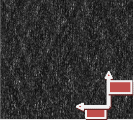
As final cases, a broader spreading function is considered, described by 30 components. In
polarization when
1
30 0 , 8 2
3 0 0 ,
varies
3
particular the noisy SAR intensity images shown in
from
00 to
3600 .
Figs. 8 and 9 are relevant to a 100 m sea peak
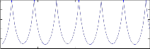
In the first sea surface simulation case a single 60 m wavelength azimuth travelling long wave is simulated and the noisy SAR intensity image is shown in Fig. 5(a). To appreciate the results an azimuth transect (see white dotted line in Fig. 5(a)) is made in the noise-free SAR image and referred to the corresponding long wave, see Fig. 5(b), where are plotted the first 200 pixels. Since an azimuth travelling wave has been si mulated, it can be experienced that the SAR imaging process is strongly non-linear in this case as clearly shown in Fig. 5(b). In fact analyzing the plots of Fig. 5(b) it is possible to recognize the non-linear effect of VB. It can be also evaluated the C parameter (section II) which, in this case, is equal to 1 witnessing a strongly non-linear imaging process. It can also be
experienced that in this case Rt(·) is equal to zero.
wavelength, range travelling, and azimuth travelling. The SAR images clearly show that a broaden spreading function has been employed. Once again it can be evaluated the C parameter, making reference to the peak wavelength and direction, recognizing that VB is a linear process in the first case and highly non-linear in the second one. And it can also be appreciated that the degree of non-linearity of the SAR imaging process decreases increasing the wind speed, as expected for fully-developed wind-seas.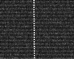
IJSER © 2011 http://www.ijser.org
International Journal of Scientific & Engineering Research Volume 2, Issue 3, March-2011 4
ISSN 2229-5518
2) When 81 , 8 2 are determined and 83 varies
from 00
to 3600
,the relationship
among 81 , 8 2 and
8 3 has been known. It can be
used to predict the critical angle
83 .
azimuth
3) It’s obviously that the effects of depolarization
can be neglected.
Fig 6
Fig 7
range
range
azimuth
[1]Kennaugh, E.M. Effects of the type of polarization on echo characteristics. In Rep.389, Antenna Lab., Ohio State Univ., Columbus, 1951.9.
[2]Jakob J.Van Zyl, Zebker. Howard A., and Charles Elachi. Imaging radar polarization signatures: Theory and observation. Radio Science, 1987, 22 (2) :
[3]R. Garello, S. Proust and B. Chapron, “2D Ocean Surface SAR Images Simulation: A Statistical Approach,” Proc. OCEANS’93, vol. 3, pp. 7-12, 1993.
A.K.Fung Scattering and depolarization on reflection of
EM waves from a rough surface. In Proc. IEEE (Communications), 1966.395-396.
[4]Gaspar R.Valenzuela. Depolarizaiton of EM Waves by
Slightly Rough Surfaces. IEEE Trans. Antennas
Propagation, 1967, 15 (4) :552-557.
[5]F. Berizzi and E. Dalle Mese. Scattering coefficient evaluation from a two-dimensional sea fractal surface. IEEE Trans. Antennas Propagation,2002, 50 (4): 426-434.
Using the 2-D ocean surface model, Huygen’s principle, Kirchhoff approximation and the neglected multiple scattering, we simulated the full polarization RCS of the ocean surface scattering fields.
The numerical results show that the full polarization scattering model coincides with other literatures. And the other conclusions as bellow:
1) The normalized radar cross section of cross polarization with significant information can’t
be neglected.
[6]Nunziata, F., Gambardella, A. and Migliaccio, M. An educational SAR sea surfacewaves simulator. International Journal of Remote Sensing, vol. 29, No. 11,
10 June 2008, 3051-3066
IJSER © 2011 http://www.ijser.org