1smkhurshedalam@gmail.com
International Journal of Scientific & Engineering Research, Volume 4, Issue 12, December-2013 1
ISSN 2229-5518
STABILITY ANALYSIS OF THIN-SHELL WORMHOLE LINEARIZED IN STRING THEORY S. M. Khurshed Alam1, N. M. Eman, M. S. Alam
Department of Physics, University of Chittagong, Chittagong, Bangladesh.
Abstract- Using the cut-and-paste technique, we construct a thin-shell wormhole by surgically grafting together two copies of spacetimes of string inspired charged black hole solution. The total amount of exotic matter in the shell needed to sustain the wormhole is calculated and its dependence with the parameters is analyzed. The dynamical stability of the stringy thin-shell wormhole is analyzed by considering the linearized fluctuation around a static solution.
PACS numbers : 04.20.Gz; 04.20.-q; 04.70.-s
—————————— ——————————
he study of traversable wormholes has received considerable attention from researchers for the past two
and half decades. Over the last two decades, there has been considerable interest in the topic of thin-shall wormholes, solution of Einstein’s field equations which act as tunnel from
Schwarzschild geometries. In this work, we study a new kind of thin-shell wormhole by surgically grafting two spacetimes of charged static black hole solution, which is often called the Gibbons-Maeda-Garfinkle-Horowitz-Strominger (GMGHS) black hole solutions. The linearized stability is analyzed under radial perturbation around a static solution. Throughout the
IJSER
one region of spacetime to another, through which a traveler
might freely pass [1-17]. It was found that these geometries,
which act as tunnels from one region of spacetime to another, posses a peculiar property, namely exotic matter, involving a stress-energy tensor that violates the null energy condition [18-20]. In fact, traversable wormholes violate all of the pointwise energy conditions and averaged energy conditions [21]. As the violation of the energy conditions is a particularly problematic issue [22], it is useful to minimize the usage of exotic matter. The null energy and averaged null energy conditions are always violated for wormhole spacetimes. As it is difficult to deal with exotic matter, it is useful to minimize the usage of exotic matter.
Visser [2], the pioneer of thin-shell wormhole, has proposed a way, which is known as ‘cut and paste’ technique,
paper we use c = G = 1.
The paper is organized as follows: In Sec. II, we construct a dynamic thin-shell wormhole by surgically grafting two spacetimes of GMGHS black hole. In Sec. III, we determine the total amount of exotic matter located at the thin- shell. In Sec. IV, we perform a detailed analysis of the stability under spherically symmetric perturbations around a static solution. Finally, conclusion of the results is given in Sec. V.
The line element of spherically symmetric and static
GMGHS black hole is given by [25]
of minimizing the usage of exotic matter to construct a
wormhole in which the exotic matter is concentrated at the
wormhole throat. In ‘cut and paste’ technique, the wormholes
ds 2 = − f (r)dt 2 + f (r) −1 dr 2 + h(r)(dθ 2 + sin 2 θdφ 2 ),
f (r ) = 1 − 2M
(1)
are theoretically constructed by cutting and pasting two manifolds to obtain geodesically complete a new one with a![]()
where
, (2)
r
throat placed in the joining shell. By invoking the Darmois-
Q2e2φ0
Israel [23] formalism, the surface stresses of the exotic matter were determined. These thin-shell wormholes are extremely
useful as one may apply a stability analysis for the dynamical
h(r ) = r
1 −
![]()
, (3)
Mr
Q2e2φ0
cases, by choosing specific surface equations of state [24]. Recently, Eiroa and Romero [6] have extended the linearized
stability analysis to Reissner-Nordström thin-shell geometries,
e− 2φ
= e− 2φ0 1 −
![]()
,
Mr
(4)
and Lobo and Crawford [4] to wormholes with a cosmological constant. Visser and Poisson [3] have analyzed the stability of thin-shell wormhole constructed by joining the two
and
F = Q sin θ dθdφ , (5)
IJSER © 2013 http://www.ijser.org
International Journal of Scientific & Engineering Research, Volume 4, Issue 12, December-2013 2
ISSN 2229-5518
where φ0 is the asymptotic constant value of the dilaton field. The metric (1), describes a black hole of mass M and
In terms of the surface energy density σ and the surface pressure p , the surface energy tensor may be written as
magnetic charge Q when the ratio Q / M
is small.
i = diag (−σ , p, p) . The thin-shell equations which is
commonly known as Einstein’s field equations then become
The thin-shell wormhole is an interesting wormhole
solution consists in applying the cut-and-past technique. We
take two copies of GMGHS black hole solution (1), removing![]()
σ = − 1 K θ , (11)
4π θ
from each spacetime the four dimensional regions is described by![]()
p = 1
8π
(K τ
+ K θ ). (12)
Ω ± = {r ±
![]()
≤ a a > r }, (6)
In the orthonormal basis
where a is a constant and rb
b
is the black hole event horizon,
{ }{ }
e , e , e
e = e , e
![]()
![]()
= (h(a))−12 e , e
= [h(a) sin 2 θ ]−12 e
τˆ θˆ φˆ τˆ τ θ
θ ϕˆ ϕ
corresponding to the GMGHS black hole solution.
to the metric (1), we obtain
To avoid the presence of an event horizon, the
±
θˆθˆ
= Kϕˆϕˆ
![]()
= ± h′(a)
2h(a)
f (a) + a 2 ,
(13)
important condition
a > rb
is applied. The removal of these
two regions result in two manifolds, geodesically incomplete,
K ± =
![]()
2a +
f ′(a)
with boundaries given by the following timelike hypersurfaces
τˆτˆ
2 f (a) + a 2
. (14)
∂Ω ±
= {r ±
![]()
= a a > r }. (7)
The components of the surface stress-energy can be deduced
IJSER
Consider the junction surface ∂Ω
as a timelike hypersurface
from Eqs. (11) and (12) as
defined by the parametric equation of the form![]()
1 h′(a) f a a
F (x µ (ξ i )) = 0. ξ i
= (τ ,θ ,φ ) are the intrinsic coordinate
σ = −
4π
h(a)
( ) + 2
, (15)
on ∂Ω , where τ is the proper time on the hypersurface. The
µ
unit normal 4-vector n to ∂Ω , is defined as![]()
![]()
−1 / 2
pθ = pφ
![]()
= p = 1
8π
h′(a)
h(a)
![]()
f (a) + a 2 + 1
8π
2a + f ′(a) .
2
(16)![]()
n = ± g αβ
∂f
∂xα
∂f
∂x β
. ∂f ,
∂x µ
(8)
f (a) + a
According to the flaring out condition the area is minimal at
with
n n µ = +1
and
µ
µ (i )
= 0.
The extrinsic curvature
the throat (then h(r) increases for r close to a and
with the two sides of the shall are defined as
h′(a) > 0 ), implies that the energy-density σ is negative at
∂ 2 x µ
∂xα
∂x β
the throat, so exotic matter is located there. The pressure p
K ± = −n
+ Γ µ ± ,
may be positive.
ij ∂ξ i ∂ξ j
![]()
αβ ∂ξ i
∂ξ j
(9)
where the ± superscripts represent the exterior and interior
spacetimes. Since the extrinsic curvature
K ij
is not
continuous across
∂Ω , so the discontinuity in the extrinsic
The total amount of exotic matter presents in the shell
curvature is defined as K ij
+ − K − . Using the Darmois-
can be quantified following [26] by the integral
Israel formalism [9], at the junction interface ∂Ω , the surface
i
![]()
Ωσ = ∫ [ρ + pr ]
− g d
3 x , (17)
stress-energy tensor S j
is obtained by the Lanczos equations
where g is the determinant of the metric tensor. We introduce
i 1 [ i
i k ]
a new radial coordinate
R = ±(r − a )
in Ω (for Ω ±![]()
S = −
j 8π
k j − δ j k k
, (10)
respectively), one obtain
2π π α
![]()
i
where k j
is the discontinuity of the extrinsic curvatures
Ωσ = ∫ ∫
∫ [ρ + pr ]
− g dR dθ dφ . (18)
across the interface ∂Ω .
0 0 −α
Since the shell is infinitely thin, the exotic matter does not
exert any radial pressure, it only exerts tangential pressure
IJSER © 2013 http://www.ijser.org
International Journal of Scientific & Engineering Research, Volume 4, Issue 12, December-2013 3
ISSN 2229-5518
and it is placed in the shell, so that
ρ = δ (R)σ
( δ is the
form of simple conservation equations. From Eq. (22), we
Dirac delta function). We therefore obtain
obtain
2π π
Ωσ = ∫ ∫ ρ
0 0
![]()
![]()
− g dθ dφ
r =a
h(a)σ ′ + h′(a)(σ + p) + {[h′(a)]2
![]()
− 2h(a)h′ (a)}
σ
2h′(a)
= 0 , (23)
![]()
2π π
where ‘′’ denotes differentiation with respect to a. If we choose
= ∫ ∫ σ
![]()
− g
r =a
dθ dφ
a particular equation of state, in the form of
p = p(σ ) , then
0 0 we can formally integrate the conservation equation and
= 4π h(a)σ (a) . (19)
Now using Eqs. (3 ) and (15), we have
obtain![]()
![]()
ln(a) = − 1 ∫ da
. (24)![]()

2M
Q 2 e 2φ0
2 σ + p
Ωσ = −2a
1 −
1 −
a
![]()
2Ma
. (20)
This relationship may then be formally inverted to yield σ
as a function of the wormhole radius,
σ = σ (a) . Thus,
Thus, the total amount of exotic matter needed is depend on
black hole mass M , magnetic charge Q and asymptotic
rearranging the terms of Eq. (15), the dynamics of the wormhole throat is completely determined by a single
constant value of the dilaton field ϕ0 . If the mass M and
charge Q of the black hole are fixed, then the total amount of
exotic matter is reduced by increasing the asymptotic constant
equation defined as
a 2 + V (a) = 0 . Here the potential
2
V (a) is
h a
value of the dilaton. Also if the magnetic charge of the black
V (a) =
f (a) − 16π 2
![]()
( ) σ (a) .
(25)
hole and the asymptotic constant value of the dilaton are kept
h′(a)
constant, then the total amoIunt of Jexotic matterSis reduced by ER
decreasing the mass of the black hole.
To perform the linearized stability analysis, choice is
to consider linearized fluctuations around an assumed static
solution characterized by the constants
a0 , σ 0
and
p0 .
Assuming this assumption, from Eqs. (15) and (16), we have![]()
Q2e2φ0 2M
The standard stability analysis method for thin-shell wormhole, based on the definition of a potential, is extended
σ = − 1
1 −
1 −
2Ma0 a0
. (26)
to our metric (1). From the Einstein’s field equations, it is easy 0
to check the energy conservation equation
2πa0
1 −
Q2e2φ0
![]()
![]()
2
Q 2 e 2φ0
Ma0
2M M
Q 2 e 2φ0
![]()
![]()
d (σ A) + p d
A = {[h′(a)]2 − 2h(a)h′ (a)}× a
f (a) + a
, (21)
1 −
![]()
![]()
1 − +
![]()
![]()
1 −
dτ dτ
2h(a)
2Ma0
a0
a0 Ma0
where
A = 4π h(a)
is the area of the wormhole throat.
p0 =
Q
1 −
2 e 2φ0
![]()
2M
1 −
. (27)
The first term in the left hand side of Eq. (23) represents the
change in internal energy of the throat and the second one is![]()
0
the work done by the internal forces of the throat, while according to the Ref. [15], the term in the right-hand side represents a flux. The above equation then may be written in
the form
A Taylor series expansion to second order in a = a0
of the potential V (a) around the static solution, yields
![]()
V (a) = V (a ) + V ′(a ) [a − a ]+ 1 V ′ (a )[a − a ]2 + O [a − a ]3 , (28)
0 0 0 2 0 0 0
d [σ h(a)] + p d [h (a)] = −{[h′(a)]2 − 2h(a)h′ (a)}× σ
. (22)
The first derivative of the potential obtained from Eq. (25) as
V (a)
can be
![]()
![]()
![]()
da da
2h′(a)
V ′(a) = f ′(a) − 32π 2σ (a) h(a) × − h(a)h′ (a)
(a) + h(a) σ ′(a) . (29)
When [h′(a)]2 − 2h(a)h′ (a) = 0, the flux term in the
![]()
![]()
h′(a)
1
[h′(a)]2 σ
![]()
h′(a)
right-hand side of Eqs. (21) and (22) is zero and they take the
Now using Eq. (23), the above equation can be written as
IJSER © 2013 http://www.ijser.org
International Journal of Scientific & Engineering Research, Volume 4, Issue 12, December-2013 4
ISSN 2229-5518
V ′(a ) =
![]()
f ′(a ) + 16π 2σ (a ) h(a ) [σ (a ) + 2 p(a)]. (30)
h′(a )
From Eq. (34) and considering V ′ (a0 ) = 0 , one can find the
The second derivative of the potential V (a) is
expression for
β 0 which is given by
2 h(a)
h(a)h′ (a)
1 −
3M
![]()
V ′ (a) = f ′ (a) + 16π
× ′
σ ′(a) +1 −
2 σ (a)
β 2 = − 1 − M × 2a0
![]()
h (a)
h(a)
![]()
[h′(a)]
![]()
![]()
0 2 a
1 −
2M
![]()
[σ (a) + 2 p(a)]+
h′(a)
![]()
σ (a)[σ ′(a) + 2 p′(a)] . (31)
a0
Q 2 e 2φ0
We now define a parameter β by the relation![]()
1 −
× Ma0
,
![]()
β 2 (σ ) ≡ ∂p
∂σ
σ . (32)
3M
![]()
1 Q 2 e
2φ0
Q 2 e
2φ0
1 Q 2 e
2φ0
![]()
(37)
The physical interpretations of β under normal
1 −
1 +
a0
![]()
![]()
2 Ma0
![]()
− + 2
Ma0 2 0
circumstances interpret as the subluminal sound speed. Here
has a simple vertical asymptote to the right of the asymptote,
we simply consider β to be a useful parameter related to the
M
M
Q 2 e2φ0
Q 2 e2φ
0
Q 2 e2φ0
equation of state. By this definition, we have
1 −
2
![]()
a 1 −
3
![]()
a 1 +
1
![]()
![]()
Ma
1
![]()
![]()
− +
Ma
> 0.
a 2
(38)
σ ′(a) + 2 p′(a) = σ ′(a)(1 + β 2 ) . (33)
0
0 2 0
0 2 0
Using Eqs. (23) and (33), we can rewrite V ′ (a) as follows
V ′ (a) = f ′ (a) − 8π 2 × {[σ (a) + 2 p(a)]2 +
Returning to the inequality V ′ (a0 ) > 0 , at the throat a = a0 , we therefore have
IJSER
3M
![]()
3
![]()
h(a)h′ (a)
2
β 2 < − 1
− M ×
![]()
1 −
2a0
![]()
2σ (a) 2 −
[h′(a)]2
σ (a) + p(a)(1 + 2β
![]()
) . (34) 0
![]()
2 a0
2M
1 −
a0
Since we are linearizing around a static solution at a = a0 , we
![]()
must have V (a0 ) and V ′(a0 ) are equal to zero. To leading
1 −
Q 2 e 2φ0
order, therefore,![]()
V (a) = 1 V ′ (a
)[a − a
]2 .
The
× Ma 0
. (39)
2 0 0
3M
1 Q 2 e 2φ0
Q 2 e 2φ0
1 Q 2 e 2φ0
configuration will then be in stable equilibrium if
V ′ (a0 ) > 0 . Now
![]()
1 −
a0
![]()
1 +
2
Ma0
![]()
![]()

+ 2
Ma 0
2
![]()
![]()
V ′ (a ) = −2a − 2 2M + M +
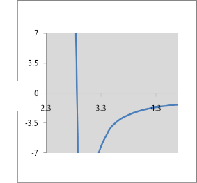
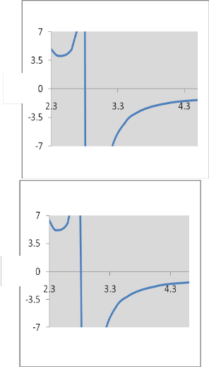
So to the right of the asymptote, the stability region of the wormhole is below the graph of Eq. (37), which is shown in
Fig. 1.
0 0 a
2M
0 a 2 1 −
![]()
a0
To the left of the asymptote, the sign of the inequality in Eq. (39) is reversed and one can obtain at a = a0
3M
1 Q 2 e 2φ0
Q 2 e 2φ0
1 Q 2 e 2φ0
1 −
![]()
1 +
a0
![]()
![]()
2 Ma0
![]()
![]()
− +
Ma0 2 0
(1 + 2β 2 ) . (35)
0
1 −
Q 2 e 2φ0
![]()
Ma0
At this order of approximation, the equation of motion of the throat is![]()
a 2 = − 1 V ′ (a
)[a − a
]2 + O[a − a
]3 . (36)
2 0 0 0
IJSER © 2013 http://www.ijser.org
International Journal of Scientific & Engineering Research, Volume 4, Issue 12, December-2013 5
ISSN 2229-5518
1 −
3M
![]()
Q / M=0.3
![]()
β 2 > − 1 −
![]()
M × 2a0
0 2 a
1 −
2M
![]()
a0
2
1 −
Q 2 e 2φ0
![]()
× Ma0
. (40) 0
2 2φ0
2 2φ0
2 2φ0
1 − 3M + 1 Q e
− Q e
+ 1 Q e
![]()
![]()
![]()
1
![]()
Ma0

2
Ma0 2 0
So to the left of the asymptote, the stability region is above the
graph. α
Fig. 1 shows typical regions of stability using
arbitrary values of the various parameters:
φ0 = 0.1,
Q / M=0.5
![]()
Q = 0 .1,
M
![]()
Q = 0.3 ,
M
![]()
Q = 0.5 , and
M
![]()
Q = 0.7 . It is
M
observed that the regions above the curves on the left and below the curves on the right are stable. The sign change is
2
determined by inequality (38). For the values![]()
Q = 0.7
and 0
M
more, the stable region above the left of the curve is not found.
This is an excellent agreement with GMGHS black hole
condition.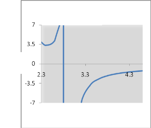
α
Q / M=0.1
Q / M=0.7
2
0
2
0
α
α
IJSER © 2013 http://www.ijser.org
International Journal of Scientific & Engineering Research, Volume 4, Issue 12, December-2013 6
ISSN 2229-5518
Fig.1: We have defined α =
2
![]()
a0 . Here we have plotted α
M
[18] M. S. Morris and K. S. Thorne, Am. J. Phys. 56, 395 (1988).
[19] M. S. Morris, K. S. Thorne, and U. Yurtsever, Phys. Rev. Lett. 61,
1446 (1988).
[20] M. Visser, Lorentzian Wormholes - from Einstein to Hawking (A. I. P.
versus β 0 . Stability regions for the thin-shell wormhole with
φ0 = 0.1 and different values of the scalar charge Q .
In this paper, we have constructed a charged thin- shell wormhole in dilaton gravity by surgically grafting two GMGHS black hole spacetimes. The surface energy density and tangential surface pressure on the shell is determined, the surface energy density is negative which ensures one of the most important criteria to construct a thin-shell wormhole. The exotic matter is localized at the thin-shell and found that the total amount of exotic matter needed is depend on black hole mass M , magnetic charge Q and asymptotic constant
value of the dilaton field φ0 and we conclude that less exotic matter is needed when magnetic charge and asymptotic constant value of the dilaton field of the black hole are increased and/or the mass of the black hole is decreased.
New York, 1995).
[21] F. S. N. Lobo, arXiv: gr-qc/0410087.
[22] C. Barcelo and M. Visser, Int. J. Mod. Phys. D 11, 1553 (2002).
[23] G. Darmois, Mémorial des Science Mathématiques, Fascicul XXV (Gauthier-Villars, Paris, 1927); W. Israel, Nuovo Cimento B 44, 1 (1966).
[24] S. W. Kim, Phys, Lett. A 166, 13 (1992); M. Visser, Phys, Lett. B
[25] A. Bhadra, Phys. Rev. D 67, 103009 (2003).
[26] K. K. Nandi, Y. –Z. Zhang, and K. B. Vijaya Kumar, Phys. Rev. D 70,
127503 (2004).
We have analyzed the dynamical stability of the thin- shell, considering the linearized radial perturbation around
the static solution at
a = a0 . The stability analysis
concentrated on the parameter β , which is a useful parameter and related to the equation of state. The parameter β 0 normally interpreted as the speed of sound and the order of magnitude is same as the speed of sound. The region of stability is obtained in terms of the mass of the wormhole M, the radius of the wormhole throat a0 and a parameter β 0 . The
2
region of stability lies β 0
Q
- α plane. It is observed that for
low values of![]()
, the stable region is significant.
M
REFERENCES
[1] M. Visser, Phys. Rev. D 39, 3182 (1989). [2] M. Visser, Nucl. Phys. B 328, 203 (1989).
[3] E. Poisson and M. Visser, Phys. Rev. D 52, 7318 (1995).
[4] F. S. N. Lobo and P. Crawford, Class. Quant. Grav. 21, 391 (2004). [5] F. S. N. Lobo, Class. Quant. Grav. 21, 4811 (2004).
[6] E. F. Eiroa and G. Romero, Gen. Rel. Grav. 36, 651 (2004). [7] E. F. Eiroa and C. Simeone, Phys. Rev. D 70, 044008 (2004). [8] E. F. Eiroa and C. Simeone, Phys. Rev. D 71, 127501 (2005).
[9] M. Thibeault, C. Simeone, and E. F. Eiroa, Gen. Rel. Grav. 38, 1593 (2006).
[10] F. S. N. Lobo, Phys, Rev. D 71, 124022 (2005).
[11] F. Rahaman et al., Gen. Rel. Grav. 38, 1687 (2006).
[12] E. F. Eiroa and C. Simeone, Phys. Rev. D 76, 024021 (2007). [13] F. Rahaman et al., Int. J. Mod. Phys. D 16, 1669 (2007).
[14] F. Rahaman et al., Gen. Rel. Grav. 39, 945 (2007). [15] E. F. Eiroa, Phys. Rev. D 78, 024018 (2008).
[16] F. Rahaman et al., Acta. Phys.Polon. B 40, 1575 (2009).
[17] F. Rahaman et al., Mod. Phys. Lett. A 24, 53 (2009).
IJSER © 2013 http://www.ijser.org