= C · adj(sE - A)B
International Journal of Scientific & Engineering Research Volume 2, Issue 4, April-2011 1
ISSN 2229-5518
Robust Impulse Eliminating Internal Model Control of Singular Systems: A Robust Control Approach
M.M. Share Pasand, H.D. Taghirad
Abstract— The problem of model based internal control of singular systems is investigated and the limitations of directly extending the control schem es for normal systems to singular ones were analyzed in this paper. A robust approach is proposed in order to establish the control scheme for singular systems, and moreover, to present a framework for robust control of singular systems in presence of modeling uncertainties. The theory is developed through a number of theorems, and several simulation examples are included and their physical int er-pretations are given to verify the proof of concept.
Index Terms— singular syst ems, Impulsive behavior, internal model control, Model based control, robust control, tracking problem, impulse elimination.
—————————— • ——————————
ingular systems represent a general framework for linear systems [1]. A singular model is an appropriate model for describing large scale interconnected systems, constrained ro- bots and other differential algebraic systems with linear alge- braic constraints [2]. Also singular models can be utilized to model a system when the dependent variable is displacement rather than time [3]. Since the first time they were introduced [4], several efforts have been made to control singular systems [5-9]. As the singular systems were firstly introduced in the state space form representation [4], they were usually studied in time domain. In [5] the problem of finite mode pole placement is studied, while simultaneous impulse elimination and robust stabilization problem is considered in [6], robust Eigen-structure assignment of finite modes is studied in [7]. In [8] strict impulse elimination is studied using time derivative feedback of the states and [9] investigated the output feedback control using a compensator. In fact most of the existing methods are exten- sions of the control schemes for standard systems [5],[6],[10]. In the singular system control context the control objectives are more complicated due to the existing obstacles such as algebraic loop phenomenon, impulsive behavior [11] , and regularity of the closed loop [8,9] . Unlike the time domain methods, there are very few works on the frequency domain control of singular systems. In the frequency domain, the tracking problem, robust control problem and impulse elimination can be treated more conveniently. Specifically the so called Internal Model Control (IMC) method provides a very interesting framework for ana- lyzing the algebraic loop, regularity of the closed loop and im-
pulse elimination problems of singular systems. Furthermore,
————————————————
• M.M. Share Pasand was graduated from KNT University of technology. He is currently within IAU Malard branch.
E-mail: momeshpa@gmail.com.
• Dr. H.D. Taghirad is a professor within the control systems group, KNT University of technology.
most of existing methods in robust control of singular systems are limited to study a special form of uncertainty. They assumed matrix E to be exactly known [6, 7 and 10]. This assumption is more restrictive than it appears, because it limits the system to be impulsive while some uncertainties may exist which lead to a strictly proper system for a singular model. Therefore this paper suggests a new concept for robust control. While previous works on robust control focuses on robust stability and robust performance, as it comes to descriptor systems, robust proper- ness of closed loop should be studied. The internal model framework for controlling singular systems provides a more logical uncertainty model and release the restrictive assumptions made in the existing state space methods for robust control of singular systems. Also it provides offset free tracking capability of the closed loop as well as being able to well treat delayed systems. The main obstacle which arises in the internal model control of singular systems is that the internal model cannot be implemeted easily, because it is generally improper. Even in computer aided control systems it is not easy to simulate a sin- gular system, since the discrete model needs future input data to determine the system state vector at the present time [1]. This problem results in an inevitable mismatch between the plant and the parallel model used in IMC.
Notice that, defining the disk shaped multiplicative uncer- tainty leads to an unbounded uncertainty profile which is not suitable in robust design of singular systems. This paper pro- vides solution to the latter problem by introducing the singular internal model filter in series with the conventional internal model filter. The aforementioned filter eases the design proce- dure, bounds the uncertainty profile. Also it makes the closed loop strictly proper and eliminates impulsive modes by smooth- ing the control action as much as needed. Another role of the introduced filter is to make it possible to design robust control- ler in the conventional context. The paper is organized as fol- lows. In the next section backgrounds are discussed and the obstacles in control of singular systems are presented, and some major limitations of the direct extension of IMC are explained. In the third section the proposed method is studied and the filter design procedure is illustrated. In the fourth section several ex-
International Journal of Scientific & Engineering Research Volume 2, Issue 4, April-2011 2
ISSN 2229-5518
amples and simulations are given to examine the algorithm both in terms of robustness properties and closed loop performance. Finally, the concluding remarks are given in last section.
As Descriptor models are a straight extension of standard state space models [1], control problem for these systems has a
and infinite respectively. Strictly proper and bi-proper systems may be generally named as proper.
CX = lim YJ (s)
s
Lemma1: A state space realization of a singular system is im- pulse free if and only if its transfer function has a nonnegative relative degree i.e. it is proper.
Proof: The transfer function matrix from input to state for sys- tem (1) can be computed as:
wider range of objectives. A control system for a standard plant is designed such that the closed loop is stable and has a prede- fined performance and acceptable robustness properties. A sin-
YJ (s) =
C (sE -
A) -1 B
![]()
= C · adj(sE - A)B
sE - A
gular control system, on the other hand, should be designed such that it is impulse free, regular and doesn’t include any al- gebraic loops in addition to the aforementioned properties. These control objectives combined with the standard objectives make the control of singular systems more challenging. Robust control of singular systems is the most challenging issue be- cause it requires robustness not only in the stability and perfor- mance but also in regularity and properness. State space robust control schemes require robust observers in order to work prop- erly and do not guarantee strict properness of the closed loop also they usually result in more complicated derivation algo- rithms. The main advantage to use internal model control scheme in here, is that the IMC provides an effective tool in frequency domain without introducing complicated methods in evaluation of closed loop performance and stability. Therefore, IMC can be regarded as a proper alternative for existing state space methods. Also IMC provides a simple framework for al- gebraic loop and properness analysis of singular control systems
It is known that degree of the nominator is equal to rank of E at
most, therefore if condition (2) is satisfied then the system trans- fer matrix will be proper and if not, the transfer matrix may be improper. On the other hand if transfer matrix is not proper con- dition (2) is not satisfied. •
Remark2: The observability assumption is essential for the above lemma .It can be shown that it may be a number of on- observable impulsive modes which do not appear in the output. Also note that condition (2) is a general condition for impulse free systems but in order to equate it with corollary 1, the obser- vability assumption is needed.
Lemma2: In the unity output feedback structure the closed loop system is strictly proper if the compensator/plant combination is strictly proper.
Proof: Expand the nominator and denominator by their respec- tive Taylor series.
which is much simpler than that in state space methods or other
I a k
s - k
frequency domain schemes. Consider the following state space
YJ ( s ) = k =1
description:
Ex = Ax + Bu
(1)
1 + I b - j
j =1
y = Cx
Definition1: System (1) is impulse free if and only if:
![]()
![]()
deg sE - A = rank E
(2)
Because CP is supposed to be strictly proper, the largest term in
its expansion has a negative power therefore the denominator has a greater degree than the nominator and thus the closed loop system is strictly proper. •
The nullity index of E is called singularity index of a singular system (1) in this paper.
Remark1: Note that the following general inequality always holds:
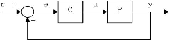
Figure1: Feedback structure
![]()
![]()
deg sE - A rank (E)
(3)
Remark3: Note that Lemma2 provides a sufficient condition. The necessary and sufficient condition is derived later. Lemma2
Corollary1: A singular system is called impulse free, if and only
if, it doesn’t exhibit impulses in its impulse response.
Definition2: A singular system is called minimal if it is observa- ble and controllable. The minimality of the plant is presumed throughout this paper.
Definition3: A transfer function is strictly proper, bi-proper and improper if the following limit is zero, a finite nonzero value
shows that why the objective of properness has not been consi- dered before the introduction of descriptor systems. Assuming strictly proper functions for plant and compensator, it is trivial that the closed loop system is strictly proper. Also for a strictly proper plant and a bi-proper compensator the closed loop will be bi-proper.
International Journal of Scientific & Engineering Research Volume 2, Issue 4, April-2011 3
ISSN 2229-5518
Lemma3: For a bi-proper plant and a bi-proper compensator, the closed loop will be improper if and only if:
~p(s) =
p(s)
![]()
D(s)
(5)
lim CP = -1
s
Lemma4: In order to have a strictly proper closed loop system with a unit feedback, if the plant is improper the compensator should be strictly proper with a sufficiently large relative de- gree.
Proof: For the closed loop to be strictly proper, the compensa- tor/plant should be strictly proper according to lemma2, there- fore the compensator should be strictly proper. •
In IMC structure the parallel model or internal model is inevitably proper or strictly proper. Therefore there always exists a mismatch between the plant and model. For a conti- nuous output especially in case of initial jumps of the input, it is required that the plant and the internal model have the
The above description for model is the most natural selec- tion for a strictly proper model, whose behavior is as close as possible to that of the plant. However, in this situation the mismatch between plant and model is not included in a disk shaped region. In other words the uncertainty bound will be infinity. Now we can take different approaches: Choose another internal model which yields bounded uncertainty; developing new theory for this kind of uncertainty; or modi- fy the plant input in order to bind the uncertainty as well as removing impulses from the response. The following lem- mas are introductory materials for the theorems developed later in this paper.
Lemma5: A control system is robustly stale, if and only if, the complementary sensitivity function fulfills the following inequality: [12]
same infinite gain and the compensator is strictly proper. This issue can be treated by a smoothing pre-filter for refer-![]()
![]()
![]()
sup YJ (s)lm < 1
(6)
ence signal but the method is not robust against model un- certainties. The IMC filter is conventionally used to enhance
Remark4: For IMC structure the complementary sensitivity
function and the uncertainty can be computed as follows:
robustness properties by victimizing closed loop response and making the compensator implementable (proper). Moreover, it accounts for online adaptation of the control system by adjusting the filter time constant. In this paper we
extend this approach by using a second IMC filter which![]()
![]()
YJ (s) = qp = qp
1 + q( p - p) 1 + qp(1 - 1/ D)
lˆ (s) = D - 1
(7)
(8)
assures the closed loop to be strictly proper and has a smooth response by compensating the singular plant impul- sive behavior. The singular internal model control filter or SIMC filter is designed to yield a continuous smooth re- sponse and a robust IMC design for singular systems. In fact by using a parallel strictly proper model in IMC, the uncer- tainty will become unbounded and the robust control will not be feasible any more. Therefore the SIMC filter has another role of bounding the uncertainty profile and making the robust control problem feasible. The disk-type uncertain- ty profile is usually assumed in robust control schemes, is described by the following relation.![]()
p( j(J)) - ~p( j(J) )
Therefore, in this case condition (6) cannot be satisfied.
Thus we need to modify the IMC structure or algorithm in order to gain a more tractable uncertainty profile. In the fol- lowing section the SIMC filter is introduced and the pro- posed method is studied.
The idea of augmenting the IMC compensator by an IMC filter can be extended to singular systems in a different manner. According to the previous discussions one way to overcome the obstacles in IMC of singular systems is to augment the compensator by an additional IMC filter, we
call it SIMC. This filter have the same structure as the con-
~p( j(J) )
![]()
lm
((J) )
lm ((J))
(4)
ventional IMC filter for step reference signals, and therefore, the IMC problem of singular systems consists of finding two
This uncertainty description allows us to incorporate several singular systems in the design while the state space uncer- tainty descriptions are limited to represent only singular systems with a pre-specified singularity index. If one aug- ments the improper plant by high frequency stable poles a strictly proper model can be obtained, which has a very close behavior to plant at least at low enough frequency range. Larger poles results in closer response to that of the plant in wider bandwidths. However, in this way the uncer- tainty becomes unbounded. In particular assume a poly- nomial of stable real poles with a unit steady state gain namely D, then one can write:
time constants; One for the conventional IMC which adjusts the closed loop performance, robustness and noise amplifi- cation; and one for the feasibility of robust control and im- pulse elimination of the singular plant. This is expectable for a singular system to require more parameters to be con- trolled, because a singular system is a general form of linear systems and cannot be treated by the same existing methods in standard systems. One advantage of SIMC is to solve the problem by introducing an additional filter without any need of complicated design procedures. Define the SIMC filter as a low pass filter:
International Journal of Scientific & Engineering Research Volume 2, Issue 4, April-2011 4
ISSN 2229-5518
f 2 (s) =
1![]()
(1s + 1)m
(9)
When there are some model inaccuracies or disturbances,
condition (12) cannot be met easily because a specific per-
Lemma6: Define SIMC filter as stated in (9), therefore the closed loop system is strictly proper, if and only if:
formance index is expected in the control objectives. In these situations a natural compromise exists and the victimization
m > -cr
(10)
of performance is inevitable. Note that one can set the IMC
filter to zero in order to satisfy (12) but this means open loop
In which, parameter cr denotes the relative degree of the
plant.
Proof: Using (9-10) as the SIMC filter, the relative degree of plant/compensator becomes strictly proper. Therefore, by means of lemma2, the closed loop system is strictly proper.
•
control of the system and therefore losing performance. The uncertainty bound generally increases with frequency. A natural routine for making the controller robust is to design a nominal H2-optimal controller according to performance specifications and then increasing the filter time constant to
meet the desired robustness properties.
Remark5: There is no need to introduce pole zero cancel-
Theorem1: Assuming
D = f -1
then there is an IMC filter
lation issues because SIMC filter cancels minimum phase
zeros of the plant at most.
Lemma7: Together with SIMC filter the singular plant is capable of being robustly controlled, if (6) can be satisfied.
such that the closed loop system is robustly stable, and fur- thermore, the system exhibits robust performance at the zero frequency, if and only if:
Proof: The new uncertainty profile have the following shape:![]()
lm (0) < 1
(13)
![]()
p pf 2 -
Proof: The IMC filter should satisfy (12) for robust stability,
because of the structure selected for IMC filter, the maxi-
lˆ (s) = D = Df - 1
(11)
mum value for the filter is unity and it occurs at zero fre-
m p 2
![]()
D
Now it is easy to choose SIMC filter such that the uncer- tainty profile is bounded.
•
quency. Therefore, for the nominal plant (12) can be satisfied only if the uncertainty upper bound is smaller than unity, and therefore, the necessary condition for the IMC filter to exist is (13). The sufficiency is obvious. •
Remark8: Note that theorem 1 is an extension of the existing
Remark 6: Note that the real uncertainty profile between
actual plant and assumed singular model is unchanged. SIMC manipulates only the mismatch between singular model and the implemented parallel strictly proper model of IMC. Also note that lˆ represents the uncertainty caused by
singular system while lm is the actual uncertainty.
Lemma8: The closed loop system with SIMC structure characterized by equations (9-11) is robustly stable, if and only if:
result in standard systems. Although the SIMC filter does not appear explicitly in the theorem, it has an essential role in the derivation of the theorem as well as lemmas. In other words, introducing the SIMC makes it possible to apply the existing frame for robust control to the singular systems.
Remark9: Theorem1 just considers the solvability of (12). In other words it studies the existence of an appropriate IMC filter which solves the robust control problem. In order to
find such an IMC filter one should increase the time con-![]()
![]()
f1 <
1
![]()
~pq~lˆ
(12)
stant and check the robust stability criterion until it is satis- fied.
Remark10: It should be noticed that there exists no con-
Proof: The complementary sensitivity function can be
stated as:
straint on the SIMC filter time constant and any positive time constant can be chosen. However when smoothness of
YJ (s) =
qp
![]()
1 + qf 2 ( p - p)
= qp = q~pD = q~f ~pDf
= q~~pf
the response is also a requirement, large time constant for
SIMC filter is required, and when a fast response is desired,
Therefore condition (6) can be states as (12).
•
Remark7: The above lemma states an essential character of SIMC, the SIMC filter caused the uncertainty to remain in a disk shaped region and the robust stability criterion is then applicable to the problem. If one studies condition (6) with and without SIMC filter, it can be seen that SIMC filter im- poses a bound on the uncertainty. Also choosing D as the inverse of SIMC filter, the uncertainty profile remains un- changed and the uncertainty caused by singular system will be zero as can be seen from (11).
it is better to choose the time constant as small as possible. Note that if the SIMC filter time constant is larger than that of IMC filter and the plant dominant time constant, it will determine the closed loop time constant. In fact the closed loop time constant is the largest time constant among the plant, IMC filter and SIMC filter time constants. Because of robustness considerations SIMC filter time constant may be smaller than IMC filter time constant, and does not restrict the closed loop performance. It is not possible to decrease SIMC filter time constant as much as desired, since input noises may be amplified.
International Journal of Scientific & Engineering Research Volume 2, Issue 4, April-2011 5
ISSN 2229-5518
Remark11: Note that (13) means that steady state gains for the plant and model should be of the same sign. A little mismatch between plant and model steady state gain may cause instability if their sign were different. This a common drawback of robust control systems for plants with zeros near the origin. By a slight change of the zero location the closed loop may become unstable if the zero is near the ori- gin.
Lemma9: Irregularity of closed loop occurs, if and only if:
shown as follows; assume that there is a plant in the family (4) that has a larger singularity index than the nominal plant. Then uncertainty profile can be written as:![]()
![]()
p - ~p lm = ~p
From the above assumption uncertainty will increase by frequency because it has an improper transfer function. Therefore, (4) cannot be satisfied as the uncertainty is un-
bounded. Moreover, for any plant being in family (4) the
cp = -1
for all s
relative degree of SIMC filter is greater than or equal to the
Proof: From the definition of regularity, a singular system is irregular if and only if:
plant singularity index and thus the closed loop system is robustly strictly proper according to lemma2. Also note that![]()
![]()
sE - A 0
(14)
regularity of the plant is guaranteed by lemma8 because of strict properness of plant/compensator combination.
In the frequency domain context of output feedback control systems the above determinant is the characteristic poly- nomial of system or the denominator of complementary sen-
sitivity function. Write the closed loop transfer function as:
The following design procedure can be followed for robust internal model control of a singular plant.
Design Procedure:
N 1. Choose the polynomial D and set
f 2 as its inverse. The
YJ (s) =
cp
![]()
1 + cp
![]()
= M =
1 + N M
N
![]()
N + M
polynomial time constant should be smaller than the domi- nant time constant of plant. According to nominal singular plant choose m such that the strictly properness of closed
According to (14) and (15) the closed loop system is irregu- lar, if and only if:
N = -M
This can be rewritten as:
loop is guaranteed.
2. For the nominal plant check the feasibility of robust con- trolhaving uncertainty profile as (4) according to (12), if sa- tisfies design IMC filter for a good performane in nominal case.
cp = -1
for all s
(15)
3. Redesign SIMC filter for having better performance if re-
The last equality also means an unsolvable algebraic loop in the simulation. •
Corollary2: For a strictly proper plant/compensator, (15)
quired.
does not occur because:
cp(s) = a s -1 + a s -2 + ....
(16)
Simulating an improper system is not possible with the
existing numerical methods, since simulation needs future data for computing the present state vector. This is why
1 2
many Papers in the field of singular systems do not include
As a result for a strictly proper compensator/plant combina-
tion the regularity issue is not of concern. This corollary de- picts the fact that why the regularity control objective is in- troduced only for singular systems and not for standard strictly proper ones.
In the following theorem we may introduce the interesting characteristics of the proposed algorithm.
Theorem2: The closed loop system with an appropriate IMC
filter designed according to (12) is robustly strictly proper
and robustly regular against all uncertainties described by
any simulation examples or just simulate causal singular systems. However, if the closed loop system is proper, any simulating software can easily implement the closed loop system regardless of the inner unsolvable loops, which form singular systems in the inner parts of the closed loop system. In this paper, some illustrative simple examples are chosen in order to show the effectiveness of the proposed algo- rithm.
Example1: Consider the nonlinear system described by the
following equations:
(4).
Proof: Note that from theorem1, the closed loop robust sta- bility and zero frequency performance are assured. The fam- ily of plants described by (4) all have a singularity index smaller than or equal to that of nominal plant. This can be
x1 = -6 x1 + 2 x2
x2 - u = 0
y = x1 + 2 x2
- u + x 2
International Journal of Scientific & Engineering Research Volume 2, Issue 4, April-2011 6
ISSN 2229-5518
The output equation is the simplest form of output equation. 12
Nonlinear output may occur in a singular system; however they are essentially treated in a similar manner. The alge-
braic part of a singular system denotes its limitations for 8
having arbitrary initial conditions. The system described by
6
(17) can be modeled by a standard state space system, too.
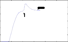
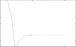
For a nominal input of u=9, the equilibrium point will be: 4
Disturbance oc cured
Disturbance rejected
x = x
= 0 x* = 3, x* = 9
2
(18)
1 2 1 2
In case of nonlinear term in (17), the nonlinearity can be con- sidered as an uncertainty, and not included in the linear model representation. The process model may be considered as a bi-proper transfer function.
0
0 10 20 30 40 50 60
Time (sec)
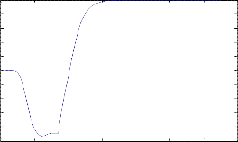
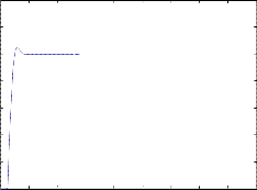
Figure 2: Set point and disturbance response
9
~p(s) =
2s + 13
![]()
(s + 6)(0.1s + 1)
![]()
p(s) = 2s + 13
(s + 6) 7
6
5
The compensator, IMC and SIMC filters may be chosen as:
4
f2 (s) =
![]()
![]()
1 = 1 3
(1s + 1) D 2
![]()
q~(s) = (0.1s + 1)(s + 6)
2s + 13 0
-1
f1 (s) =
1
![]()
(0.5s + 1)
0 10 20 30 40 50 60 70
Time (s ec)
Figure 3: Set point response with initial condition
Closed loop system responses to different inputs with dif- ferent initial conditions are shown in figures 1 to 3. Before change in the set point, initial condition is vanished and then the set point signal is tracked without any off set. The closed loop system is stable as the phase portrait shows and as it is strictly proper, a smooth response is attained. Closed loop system is able to follow any piecewise constant refer- ence signal and reject constant disturbances. The main ad- vantage of the presented control structure is to make closed loop, impulse free, even strictly proper, in a robust manner, i.e. regardless of uncertainty in the plant model.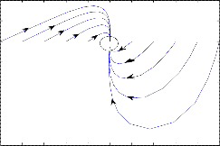
0.4
0.2
0
-0.2
-0.4
-0.6
-0.8
-1
-5 -4 -3 -2 -1 0 1 2 3 4 5
6
5
4
3
2
1
0
-1
-2
0 10 20 30 40 50 60 70
Time (sec)
Figure 1: System response to initial condition
The fading character of the output is due to guaranteed sta- bility of the closed loop system. Figure2 shows the system response to a reference input of magnitude 9, combined with a disturbance. It shows the system capability to reject dis-
X1
Figure 4: phase portrait of closed loop near the origin
This example shows that the closed loop system is strictly proper regardless of any model uncertainties while bounded and also it provides an example of robust stability and zero frequen- cy performance design.
Example2: Consider a group of linear singular systems as described by the following set of transfer function.
p(s) = s 2 + CXs + 1 p (s) = s 2 + 3s + 1 p ( s) = s 2 + 4s + 1 p (s) = s 2 + 1
The nominal plant (model) is assumed to be:
~ 2
turbances.
p(s) = s
+ 2s + 1
The parallel model and compensator are:
International Journal of Scientific & Engineering Research Volume 2, Issue 4, April-2011 7
ISSN 2229-5518
~p(s) =
![]()
s 2 + 2s + 1 (0.1s + 1)3
1.4
1.2
1
![]()
q(s) = f (s) (0.1s + 1)
1 s 2 + 2s + 1
0.8
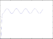
It is aimed to design a single robust controller for all plants described above. The uncertainty norm is bounded for all of the models described in (19), however, its infinity norm is near the unity for case p4. Following figures depict closed loop behavior in tracking step set point. Set point tracking is almost perfect even in presence of uncertainties. This charac- teristic also exists in conventional unit feedback control, e.g. PID controllers. However state space methods like [5] don’t include this feature. In contrast to the aggressive nature of singular systems, closed loop response is smooth enough to ensure preventing any damage to the instruments. In the last case the oscillating behavior of plant is not included in the model and therefore closed loop response is not satisfactory. Note that while steady state gains of plant and model have the same sign, the closed loop is robustly stable. And while the uncertainty is bounded it is robustly strictly proper.
1.4
1.2
0.6
0.4
0.2
0
0 50 100 150 200 250
Time (sec)
Figure 7: Step response for p3
In this paper a new, effective and simple control scheme is proposed for robust internal model control of singular linear systems. The method has many advantages over the exist- ing, state space methods including robust strict properness of the closed loop, avoiding algebraic loops, robust tracking of specific signals and the ability to robustly stabilize a larg- er group of singular systems comparing with other methods. Two simulation examples are included to depict the algo- rithm performance.
1
0.8
0.6
0.4
0.2
0
1.4
1.2
1
0.8
0.6
0.4
0.2
0
0 20 40 60 80 100 120 140 160 180 200
Time (sec)
Figure 5: step response for p1
[1] Mertzios, B.G. and F. Lewis, “Fundamental matrix of discrete singular systems”, Journal of circuits, systems and signal processing, vol.8, NO.3,
1989.
[2] Dai, L. “Singular control systems”, Springer verlag, 1989.
[3] Campbell, S.L, R. Nikoukhah and B.C. Levy, “ Kal man filtering for general discrete time linear syste ms”, IEEE transactions on automatic control, vol.44, NO.10, pp. 1829-1839,1999.
[4] Luenberger, D. “Dyna mic e quations in descriptor form”,IEEE
transactions on automatc control, vol.AC.22, NO.3, June, 1977
[5] Syrmos, V.L. and F.L. Lewis, “Robust eigen value assignment in generalized systems”Proceedings of the 30th conference on decision and control, England, 1991.
[6] Fang, C.H., L.Lee and F.R. Chang, “Robust control analysis and design for discrete time singular systems”, Automatica, Vol.30, NO.11, pp.1741-
1750, 1994.
[7] Xu, S. , C. Yang, Y. Neu and J. Lam, “Robust stabilization for uncertain discrete singular systems”, Automatica, Vol.37, pp.769-774, 2001.
[8] Mukundan, R. and W. Dayawansa, “Feedback control of singular systems- proportional and derivative feedback of the state”, International journal of systems science, vol.14, NO.6, pp.615-632, 1983.
[9] Chu, D.L., H.C. Chan and D.W. Ho, “ Regularization of singular syste ms by derivative and proportional output feedback”, Siam journal of matrix nalysis and applications, vol.19, NO.1, pp.21-38, January, 1998.
[10] Xu, S. and J. Lam, ” Robust stability and stabilization of discrete singular
0 20 40 60 80 100 120 140 160 180
Time (sec )
Figure 6: Step response for p2
systems: An equivalent characterization”, IEEE transaction on automatic
control, vol.49, NO.4, April 2004.
[11] Hou, M. “Controllability and elimination of impulsive modes in descriptor systems”, IEEE transactions on automatic control, vol.49, NO.10, 2004.
[12] Morari, M. and E. Zafiriou, “Robust process control”, Prentice Hall, 1989.