gravitational and frictional forces.
The Newton-Euler recursive algorithm of the inverse dynamics is as follows:
International Journal of Scientific & Engineering Research, Volume 6, Issue 2, February-2015 166
ISSN 2229-5518
Robotic Configuration for Paralyzed Swing Leg with Motion Captured Stance Hip Orientation
A. Chennakesava Reddy, B. Kotiveerachari, P. Rami Reddy
—————————— ——————————
UMAN walking is a smooth, highly coordinated, rhythmical movement by which the body moves step by step in the desired direction. Numerous studies from
various fields, such as biomechanics, robotics, and
ergonomics, have provided a rich database on normal
straight-walking gait patterns. The human beings experience
heart attack and spinal cord injury. Mutilation in walking
ability after such neurological injuries is general. The clinical
stepping motion training is inadequate because the training is labor concentrated. Many therapists are mandatory to control the pelvis and legs. A locomotion rehabilitation called body weight supported (BWS) training has shown warranty in enhancing locomotion after spinal cord injury [1]. The technique involves suspending the patient above a treadmill to partly relieve the body weight, and physically supporting the legs and pelvis while moving in a walking pattern. Patients who be given this therapy can considerably increase their independent walking ability [2, 3]. This technique works by force, position, and touch sensors in the legs during stepping in a repetitive manner, and that the circuits in the nervous system learn from this sensor input to generate locomotion.
.
This article explores an alternate approach toward generating strategy for developing dynamic motion planning for walking and training the paralyzed leg with a robot attached to the pelvis. The robotic configuration used is paralyzed swing leg with motion captured stance hip orientation. This configuration is studied to control the swing leg by applying a normative pelvis trajectory.
Human walking requires the simultaneous involvement of all lower limb joints in a complex pattern of movement. Basically, all normal people walk in the same way. From human gait observations [4], the differences in gait between one person and another occur mainly in movements in the coronal and transverse planes. Throughout the whole body, those joint movements that occur in the sagittal plane are very similar between individuals, and if the upper limbs are unencumbered, they actually demonstrate a stereotyped pattern of reciprocal movement in phase with the lower limbs. The word configuration is taken from the human gait terminology.
The BWS training with robotics is an attractive as it improves the training. A difficulty in automating BWS training is that the required amount of forces at the pelvis and legs are unknown.
————————————————
• Professor, Department of Mechanical Engineering, JNTUH College of
Engineering, Kukatpally, Hyderabad – 500 085, Telangana, India
acreddy@jntuh.ac.in, 09440568776
• Professor, Department of Mechanical Engineering, National Institute of
Technology, Warangal, Telangana, India
• Former Registrar, JNT University, Kukatpally, Hyderabad – 500 085, Telangana, India.
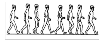
While walking, the position and orientation of legs change as shown in figure 1. The robot used to assist the paralyzed leg should simulate the walking pattern of the normal leg. Thus, the rehabilitation robot configuration is defined [5]. The rehabilitation robot is described kinematically by giving the values of link length, link twist, joint distance and joint angle. The rehabilitation robot transformation matrices are very vital for the dynamic analysis.
IJSER © 2015 http://www.ijser.org
International Journal of Scientific & Engineering Research, Volume 6, Issue 2, February-2015 167
ISSN 2229-5518
gravitational and frictional forces.
The Newton-Euler recursive algorithm of the inverse dynamics is as follows:
• Initialization
Fig. 1 Change of position and orientation of legs during walking
V0 ,V0 , Fn+1
• Forward recursion: i = 1 to n
Vi = Ad −1 Vi−1 + Si qi
i −1,i
Vi = Ad −1 Vi−1 + Si qi + ad v Si qi
i −1,i
• Backward recursion: i = n to 1
(4) (5)
(6)
* * *
Fi = Ad −1 Fi+1 + J iVi − ad v + J iVi − ad v J iVi (7)
i −1,i
τ i = S T Fi + f ci sgn(qi ) + f vi qi
(8)
In the algorithm, the index i represents the ith link frame counted from the base frame (i = 0). The joint screw, spatial velocity, spatial acceleration and spatial force are written as S,
V , V and
F � se(3) , respectively. Particularly, V0
and
V0
represent the spatial velocity and acceleration of the base, respectively, while Fn+1 represents the external spatial force
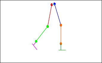
Fig. 2. Rehabilitation robot to represent normal legs.
on the last link or end-effector.
Ti 1,i
� SE(3)
denotes the
transformation from the (i – 1)th link frame to the ith link frame. The joint velocity, acceleration, force and the Coulomb
The position and orientation of frame i relative to that of frame
(i–1) is given by
and viscous frictions are written as q , q , τ , fc and
respectively. And J is the spatial inertia matrix
fv � ,
2
T0,n (q1,q2,.....qn ) = T0,1(q1 )T1,2 (q2 ) .... Tn −1,n (qn )
(1)
J = I i − mi rˆi
mi rˆi
where qi is the joint variable for link i.
− mi rˆi
mi • 1
(9)
The mapping between the joint velocities and the end-effector
where mi and Ii are the mass and inertia of the ith link,
respectively; ri is a vector from the origin of the ith link frame
velocities is defined by the differential kinematics equation
to the center of mass of ith link;
rˆi is the skew symmetric
ω
Ve =
= J e (q )q
matrix formed by ri using the notation from the last chapter;
ve
(2)
and 1 is an identity matrix. The spatial velocity and force are
wi
where Ve is the spatial velocity of the end-effector; we and ve
the angular and linear velocities of the end-effector, respectively; q the generalized velocity of the robot
Vi = v
i
manipulator; and Je the Jacobian matrix. The Jacobian can be
m
Fi =
ti
expressed entirely in terms of the joint screws mapped into the
f ti
(10)
base frame. Each column of
J s (q) depends only on q1, q2, . . .
where w, v, mt and ft are the angular velocity, linear velocity,
qi-1. In other words, the contribution of the ith joint velocity to the end-effector velocity is independent of the configuration in the manipulator.
The dynamic equations of open-chained robot manipulators can be expressed in the general form
moment and force, respectively. This recursive formulation shows how the spatial velocity and acceleration propagate forwards from the base to the end-effector and how the spatial force propagates backwards from the end-effector to the base.
The B-spline curve is used to the joint trajectories [6]. The B-
H (q)q + h(q, q ) = τ
(3)
spline curve, q ∈ ℜ is written as
which relates the applied joint forces τ to the joint positions q
and their time derivatives q and q . H(q) is the mass or inertia
m
q(t, p) = ∑ p j B j,k (t )
j =0
(11)
matrix and
h(q, q )contains the centrifugal, Coriolis,
IJSER © 2015 http://www.ijser.org
International Journal of Scientific & Engineering Research, Volume 6, Issue 2, February-2015 168
ISSN 2229-5518
where
p = {p 0 ,...p m } , with , are the control points and
B j ,k is
the B-spline basis function. The index k defines the order of
the basis polynomial, e.g. k = 4 for a cubic one or k = 6 for a
quintic one. The semi-infinite constraints are transformed into
a set of linear inequalities by exploiting the convex hull
property [7].
Passive torque-angle properties of the hip, knee, and ankle joints were measured for the subject with a Biodex active dynamometer. The dynamometer imposed slow iso-velocity movements at the joints and measured applied torques and resulting joint angles. Joints were measured in a gravity- eliminated configuration. The dynamic properties of the human model is given in Table 2.
TABLE 2
Dynamic Properties of Human Model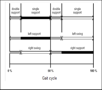
Fig. 3. Gait cycle of human walking
4 HUMAN MODEL AND WALKING MOTION
For studying the motion of the legs, the head, torso, pelvis, and arms were combined into a single rigid body (upper trunk). The walking gait cycle (figure 3) was assumed to be bilaterally symmetric [7]. The left-side stance and swing phases were assumed to be identical to the right-side stance and swing phases, respectively. Thus, only one-half of the gait cycle was simulated in this study. The stance hip was modeled as a two degrees-of-freedom (DOF) universal joint rotating about the x- and y-directions. The upper trunk was fixed about the z-axis. The swing hip was modeled as a 3 DOF ball joint rotating about axes in the x-, y-, and z- directions. The knee and ankle were modeled as 1 DOF hinge joints about the z-axis.
Motion capture data of major body segments for an unimpaired person during treadmill walking was obtained using a video-based system at FESTO Pvt.Ltd, Bangalore. The
The joints were modeled as nonlinear springs in which the joint torque was a polynomial function of the joint angle. A least squares method was used to best-fit polynomials. Third order polynomial function was used for the torque-angle property of each joint. A polynomial of order 7 is used to the ankle joint data. The resulting polynomial equations for curves are mentioned as follows:
frequency of motion capture was 50 Hz. External markers
were attached to the body at the antero-superior iliac spines
(ASISs), knees, ankles, tops of the toes, and backs of the heels
Hip external/internal rotation (− 600 ,600 )
τ m = −0.6837 − 0.7621q + 0.9772q 2 − 2.2620q3
(12)
[8, 9]. The link lengths and joint orientations are shown in
Table 1. The human subject was 1.95 m tall and weighed 70 kg.
Hip abduction/adduction (− 50 0
,30 0 )
τ m = −0.0542 − 0.8266q − 6.0205q 2 − 29.0271q 3
(13)
TABLE 1 0 0
Link Lengths
Hip extension/flexion (− 35 ,70 )
τ m = 1.0863 + 1.5721q + 6.3488q 2 − 23.0405q3
(14)
IJSER © 2015 http://www.ijser.org
International Journal of Scientific & Engineering Research, Volume 6, Issue 2, February-2015 169
ISSN 2229-5518
Knee flexion/extension (− 1400 ,00 )
The function τ sd
is C2 continuous in order to be used in
τ m = −24.9343 − 53.1584q − 37.5211q 2 − 9.8685q3
Ankle plantar/dorsal flexion (− 520 ,460 )
τ m = 0.1305 − 3.99564q + 1.5596q2 − 4.7881q3 + 2.4229q4
+ 6.2372q5 − 5.6802q6 − 19.5304q7
(15)
(16)
the computation of the analytical gradient in the dynamic
motion optimization. Four steps at three different treadmill
walking speeds (1.75, 1.25 and 0.75 m/sec) were obtained
from motion capture.
In addition to the polynomial function, a nonlinear spring- damper system was used to place a hard limit on joint movement when it is close to its upper and lower bounds.
The swing hip, knee and ankle joints were set to be passive while the stance hip joint followed the trajectory identified from motion capture. Assuming no ground contact, the equations of motion were solved. Figure 4 shows that the
swing leg moves at its natural frequency. Solid lines represent
− β (10 4 (q − q ) + 5x10 2 q )
if q ≥ q2
the simulated data. The dashed lines signify experimental
τ sd
= − β (10 4
(q − q1 ) + 5x10 2
q )
if q ≤ q1
data. However, there would be a collision between the leg and
0
where
otherwise
(17)
the ground at about x = 0 (mid-stride) if the ground were not
neglected. The leg is internally rotated away from the desired
configuration at the end of swing as shown in figure 5.
6 x10⁵ (q − q2 )5 − 1.5x10⁵ (q − q2 )4 + 10 4 (q − q2 )3
β = − 6 x10⁵ (q − q )5 − 1.5x10⁵ (q − q )4 + 10 4 (q − q )3
if q2 + 0.1 ≥ q ≥ q2
if q − 0.1 ≥ q ≥ q
1 1
1
1 1 1
otherwise
Fig. 5. Gait for duration of 0.60 sec
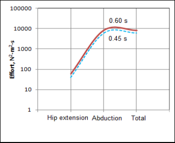
The applied effort for two gait durations is shown in figure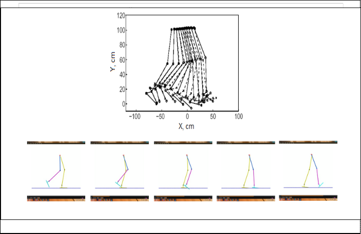
6. The effort required for step duration of 0.60 seconds is higher than that required for 0.45 seconds. This shows that
IJSER © 2015 http://www.ijser.org
Int , February-2015 170
ISS
Fig. 6. Applied effort for step durations
most of the effort goes into tilting the pelvis, i.e. abducting the stance hip, due to working against gravity.
Walking motion was generated for a robot attached to the pelvis of a paralyzed person suspended on a treadmill. A leg swing motion was created by moving the pelvis. Although it may not be possible to fully control swing by manipulating the pelvis, a surprising amount of control is possible, and the level of control appears sufficient for achieving repetitive stepping for a paralyzed person. The dynamic motion planning can also generate leg swing motions similar to the human gait during the swing phase.
The prospective work is divided into the following interesting areas:
• Build a robot for body weight supported training. The resulting motions found with the dynamic motion planner can be tested on the robot. That would provide useful information to modify the current motion planner and improve the design of the robot.
• Generate a complete walking gait. In this work, the stepping motion has been generated only during the swing phase of a gait. However, the effort applied to the stance leg is not taken into account in this work. This has to be done in order to generate a complete gait.
[1] I. Wickelgren, “Teaching the spinal cord to walk”, Science, Vol.279, pp.319–321, Jan 1998.
[2] H. Barbeau, K. Norman, J. Fung, M. Visintin, and M. Ladoucer,
“Does neuro-rehabilitation play a role in the recovery of walking in neurological populations”, Annals New York Academy of Sciences, Vol.860, pp.377–392, November 1998.
[3] H. Ko, and N.I. Badler, “Straight-line walking animation based on
kinematic generalization that preserves the original characteristics”,
Graphics Interface, Vol.28, pp.9-16, 1993.
[4] M. P. Murray, A. B. Drought, and R. C. Kory, “Walking patterns of normal men”, Journal of Bone and Joint Surgery, Vol.46A, pp. 335-
359, 1964.
[4] A.C. Reddy, “Studies on synthesis and optimization of robotic
configurations used for training of paralyzed person through dynamic parameter consideration”, Ph.D Thesis, 2007.
[5] A.C. Reddy, B. Kotiveerachari, P.R.Reddy, “Dynamic trajectory planning of robot arms”, Journal of Manufacturing Technology, vol.3, no.3, pp.15-18, 2004.
[6] Chennakesava R Alavala, “CAD/CAM: Concepts and Applications”.
PHI Learning Private Limited, New Delhi, 2008.
[7] A.C. Reddy , B. Kotiveerachari, “Different methods of robotic motion planning for assigning and training paralysed person”, Journal of Institution of Engineers, vol. 88, no.2, pp.37-41, 2008.
[8] A.C. Reddy, G.S. Babu, “Dynamic mechanisms of kneecap, compliant ankle and passive swing leg to simulate human walking robot”, International Journal of Advanced Mechatronics and Robotics, vol.3, no.1, pp.1-7, 2011.
IJSER © 2015 http://www.ijser.org