International Journal of Scientific & Engineering Research, Volume 3, Issue 2, February-2012 1

ISSN 2229-5518

Reliability Analysis of a Cold Stand By System with Repair-Equipment Failure and Appearance and Disappearance of Repairman with Correlated Life Time

Mohit Kakkar , Ashok Chitkara ,Sanjeev Kumar

Abstract - The aim of this paper is to present a reliability analysis of a two unit cold standby system with the assumption that the repair- equipment may also fail during the repair of a failed unit. There is only one repair facility which may be appeared and disappeared randomly. Failure and Repair times of each unit are assumed to be correlated. Using regenerative point technique various reliability characteristics are obtained which are useful to system designers and industrial managers. Graphical behaviors of MTSF and profit function have also been studied.

Keywords - Transition Probabilities, sojourn time, MTSF, Availability, Busy Period, Profit Function, Bivariate exponential distribution.

1. INTRODUCTION

——————————  ——————————

single repair facility. When repair equipment fails during the repair of any failed unit, repairman starts

A two identical unit cold stand by systems have widely studied in literature of reliability theory, repair maintenance is one of the most important measures for increasing the reliability of the system. Many authors have studied various system models under different repair policies [1-4] they have assumed that the failure and repair times are uncorrelated random variable. They have also assumed that the repair –equipment used for repairing a failed unit can never failed but in real life this is not so. It is also possible that the repair- equipment may fail for some reason during repair process of a failed unit in this case repairman first repairs the repair-equipment and repairman also need rest so repairman can appear and disappear randomly. Taking this fact into consideration in this paper we investigate a cold stand by unit system model assuming the possibility of failure of repair-equipment during the repair process of a failed unit with appearance and disappearance of repairman with failure and repair of unit as correlated random variables having their joint distribution as bivariate exponential .

2. SYSTEM DESCRIPTION

System consists of two identical units one is operative and other is in cold stand by. There is

the repair of failed unit and repair equipment may also fail. The joint distribution of failure and repair times for each unit is taken to be bivariate exponential having density function. Each repaired unit works as good as new.

3. NOTATIONS

For defining the states of the system we assume the following symbols:

:

International Journal of Scientific & Engineering Research, Volume 3, Issue 2, February-2012 2

ISSN 2229-5518

Yi(i=1): Random variables representing the repair times of A unit

p21 

p 

1 (1  r1 )  x

1 (1  r1 )

fi(x,y): Joint pdf of (xi,yi);i=1

   (1  r )ei x  i y I (2 (  r xy ); X , Y , ,   0;

0  ri  1,

 (  r xy) j

p31

1 (1  r1 )  x

 

1 (1  r1 )  

whereI0 (2 i i ri xy )  

j 0

i i i

( j !)2

p34

 1 (1  r1 )

ki(Y/X): Conditional pdf of Yi given Xi=x is given by

=  ei ri xi y I (2 (  r xy )

 (1r ) x

p51

’,

1 (1  r1 )  

 (1  r )

 1 1

1 (1  r1 )    

gi(.): Marginal pdf of Xi= i (1 ri )e
hi(.): Marginal pdf of Yi= i (1 ri )e

i i

 i (1ri ) y

p54 



1 (1  r1 )    



qij (.), Qi

pdf &cdf of transition time from
regenerative states pdf &cdf of
transition time from regenerative state Si
to Sj.

p56 

1 (1  r1 )    

(1-12)

i :

Mean sojourn time in state Si.

p01  1

 : Symbol of ordinary Convolution

p  p

 p  p  1

t 10 12 15 13

A(t ) 

B(t )   A(t  u)B(u)du

p  p

 p  p  p  p  1

: symbol of stieltjes convolution

10 12 13 14.5 16.5 11.5

p21  p26  1

t p  p  1

21 26.5

A(t )

B(t)   A(t  u)dB(u)

p  p  1

0 31 34

p51  p54  p56  1

3.1 Transition Probability and Sojourn Times

The steady state transition probability can be as follows

p45  1

p65  1

p01  1 ,

0  ,

p10

 1 (1  r1 )

1 (1  r1 )  1 (1  r1 )    

1 

1 (1  r1 )

p15

 1 (1  r1 )

1 (1  r1 )  1 (1  r1 )    

p12 

1 (1  r1 )  1 (1  r1 )    



2 

1 (1  r1 )  x

, 3

  1 (1  r1 )

p13 

1 (1  r1 )  1 (1  r1 )    



1 (1  r1 )  1 (1  r1 )    

4 

1   1

 , 8 x

(13-27)

4. ANALYSIS OF CHARACTERISTICS

International Journal of Scientific & Engineering Research, Volume 3, Issue 2, February-2012 3

ISSN 2229-5518

4.1 MTSF (Mean Time to System Failure)

We get

A* (s)  N1 (s)

To determine the MTSF of the system, we
regard the failed state of the system as
absorbing state, by probabilistic arguments, we

D1 (s)

The steady state availability is A 
(43)
(sA* (s))  N1

0 lim 0 D

get

0 (t )  Q01

1 (t )

Where

s0 1

1 (t )  Q10

0 (t )  Q13

3 (t )  Q12

2 (t )  Q15

N1  0 p12 [ p21 (1  p45 p54 )  p25.6 p51 ]  0 p13 [ p31 (1  p45 p54 )  p34 p45 p51 ]

0 [1  p11.5  p16.5 p51 )  p45 p54 (1  p11.5 )  p14.5 p51 ]

2 (t )  Q21

1 (t )  Q26

 p p [ p p

 (1  p

)  p p

]  p p p [ p      p ]

3 (t )  Q31 (t )

1 (t )  Q34

0 56 65 31 13 11.5 12 21 01 51 65 13 3 1 2 12

 p01 p12 2 [(1  p45 p54 )]  p01 1[(1  p45 p54 )]  p01 p13 3 [(1  p45 p54 )]

(28-31) Taking Laplace stieltjes transforms of these relations and solving for 0 (s) ,

 ** (s)  N (s)

D1  0 p10 p51  1 p51  2 p12 p51  3 p13 p51  4 (1  p10  p11.5  p13 p31  p12 p21 )

(4 p54  6 p56 )(1  p12 p21  p13 p31  p11.5 )  4 ( p13 p34 p51  p14.5 p51 )  6 ( p10 p56 )

(44-46)

Where

D(s)

(32)

4.3 Busy Period Analysis of the Repairman

Let Bi(t) be the probability that the repairman is busy at instant t, given that the system entered regenerative

N  0 (1  p12 p21  p13 p31 )  1 p12  3 p13

D  1  p10  p12 p21  p13 p31 

state I at t=0.By probabilistic arguments we have the following recursive relations for Bi(t)

B0 (t)  q01 (t)  B1 (t)

B1 (t)  W1  q10 (t)  B0 (t)  q12 (t)  B2 (t)  q13 (t)  B3 (t)  q14.5 (t)  B4 (t) 

(33-34)

q (t)  B (t)  q

(t)  B (t)

4.2 Availability Analysis

Let Ai (t) be the probability that the system is in up-

16.5 5 11.5 1

B2 (t)  W2  q21 (t)  B1 (t)  q25.6 (t)  B5 (t)

B3 (t)  q31 (t)  B1 (t)  q34 (t)  B4 (t)

B4 (t)  q45 (t)  B5 (t)

B5 (t)  W5  q51 (t)  B1 (t)  q56 (t)  B6 (t)  q54 (t)  B4 (t)

state at instant t given that the system entered

B (t)  W  q

(t)  B (t)

regenerative state i at t=0.using the arguments of the
theory of a regenerative process the point wise

6 6 65 5

(47-53)
availability

Ai (t) is seen to satisfy the following

Taking Laplace transform of the equations of busy

recursive relations

period analysis and solving them for B0 (s) ,we get

B* (s)  N2 (s)

A0 (t )  M 0 (t )  q01 (t )  A1 (t )

A1 (t )  M1 (t )  q10 (t )  A0 (t )  q13 (t )  A3 (t )  q12 (t )  A2 (t )  q14.5 (t )  A4 (t )

D1 (s)

(54)

q16.5 (t )  A5 (t )  q11.5 (t )  A1 (t )

A2 (t )  M 2 (t )  q21 (t )  A1 (t )  q25.6 (t)  A5 (t)

In the steady state

A3 (t )  M 3 (t )  q31 (t )  A1 (t )  q34 (t )  A4 (t )

A4 (t )  q45 (t )  A5 (t )

A5 (t )  q51 (t )  A1 (t )  q56 (t )  A6 (t )  q54 (t )  A4 (t )

B  (sB* (s))  2

s0 1

Where
(55)

A6 (t )  q65 (t )  A5 (t )

N   [ p

 p p p

]   p p [ p p

 (1  p p ]

2 1 01 01 45 54 01 56 65 2 01 12 45 54 56 65

(35-42)

 [ p p p

 p p p p

 p p p

 p p ]

Now taking Laplace transform of these equations and

5 01 12 25.6 01 13 34 45 01 45 14.5 01 16.5

6 [ p01 p12 p25.6 p56.7 p01 p13 p34 p45 p56  p01 p56 p45 p14.5  p01 p56 p16.5 ]

(56)
solving them for

A0 (s),

D1 is already specified.

International Journal of Scientific & Engineering Research, Volume 3, Issue 2, February-2012 4

ISSN 2229-5518

4.4 Expected Number of Visits by the Repairman

We defined as the expected number of visits by the repairman in (0,t],given that the system initially starts from regenerative state Si

By probabilistic arguments we have the following recursive relations for Vi (t)

Taking laplace stieltjes transform of the equations of expected number of visits And solving them for V ** (s) , we get

V0 (t )  q01 (t )  (1  V1 (t))

V1 (t )  q10 (t )  V0 (t)  q12 (t)  V2 (t)  q13 (t)  V3 (t)  q14.5 (t)  V4 (t) 

q16.5 (t )  V5 (t )  q11.5 (t )  V1 (t )

V2 (t )  q21 (t )  V1 (t )  q25.6 (t)  V5 (t) V3 (t )  q31 (t )  V1 (t)  q34 (t)  V4 (t) V4 (t )  q45 (t )  V5 (t )

V5 (t )  q51 (t )  V1 (t)  q56 (t)  V6 (t)  q54 (t)  V4 (t)

V6 (t )  q65 (t )  V5 (t )

V ** (s)  N3 (s)

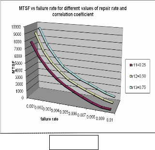
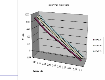
6. CONCLUSION For a more clear view of the

system characteristics w.r.t. the various parameters involved, we plot curves for MTSF and profit function in figure-2 and figure-3 w.r.t the failure parameter ( 1 ) of unit A for three different values of correlation coefficient (r11 =0.25, r12 =0.50, r13 =0.75), between X1 and Y1 while the other parameters are kept fixed as

  .005, 1  .03,  .001,  .04

x  .05, C0  500, C1  300, C2  50

From the figure-2 it is observed that MTSF decreases as failure rate increases irrespective of other parameters. the curves also indicates that for the same value of failure rate,MTSF is higher for higher vaues of correlation coefficient(r),so here we conclude that the high value of r between failure and repair tends to increase the expected life time of the system.
From the figure-3 it is clear that profit decreases linearly as failure rate increases. Also for the fixed value of failure rate, the profit is higher for high

D1 (s)

In steady state
(57-65)
correlation (r).

REFERENCES

V  (sV * (s))  N3

0 lim 0 D

1.Said K.M.EL, Salah M, Sherbeny EL (2005) “Profit

analysis fof a two unit cold standby system with

s0 1

Where
(66)
preventive maintenance and random change in Units”,
1(1):71-77, 2005, ISSN 1549-3644 (2005).

N3  p01 p12 p21[ p45 p54  p65 p56 ]  p01 p12 p51 p25.6  p01 p12 p45 p25.6  p01 p13 p45 p34 p56 p65

 p01 p14.5 p45 p45 p56 p65  p01 p16.5 p45 p54

(67) D1 is already specified

5. PROFIT ANALYSIS

The expected total profit incurred to the system in steady state is given by

2.Goyal,V.and murari,K.(1984). “Cost analysis of two- unit standby system with regular repair man And patience time”, microelectron.reliab.vol.4 no.3, pp.453-

459.

3.Goel, L.P. R.Gupta, and Singh, S.k.(1985) “cost analysis of two-unit priority standby system with imperfect switch and Arbitrary distribution”, microelectron.reliab.vol.25 no.1, pp. 65-69.

3.Goyal,V. and Murari,K.(1984) “cost analysis of a two unit standby system with regular repairman and

P  C0 A0  C1B0  C2V0

Where

C0 =revenue/unit uptime of the system

(68)
patience time”,microelectron.reliab.vol.25 no.1,pp. 453-
459.

4.Goel,L.P. and Gupta,R.(1990) “Cost benefit analysis

of two unit parallel system with administrative delay
in repair”,Int.j.of system science,vol.21,pp.1369-1379

C1 =cost/unit time for which repairman is busy

C2 =cost/visit for the repairman

5.Kumar,A and lal,P.(1979). “Stochastic behavior of a two unit satnd by system with constant failure And intermittently available repair facility”, int.J.systems sciences, vol.10 no.6, pp.589-603.

International Journal of Scientific & Engineering Research, Volume 3, Issue 2, February-2012 5

ISSN 2229-5518

Transition Diagram

S0

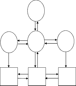
Ao , As

S2

Afw,Ao

Mfr

θ

g(t)

X1 Y1

S1

Afr,Ao ∅

ω

S3

Afw,Ao

X1 X1 Y1 X1

FIGURE -1

S6

Afw,Afw

Mfr

θ

g(t)

S5

Afr,Afw ∅

ω

S4

Afw,Afw

Mohit Kakkar

Research Scholar,
Chitkara University, Himachal Pradesh, India.

Ashok Chitkara

International Journal

ISSN 2229-5518

of Scientific &

Engineering

Research,

Volume 3, Issue 2, February-2012

Sanjeev kumar

Asst. Professor,

Piet ,Panipat Haryana,India

h t t p ://www.ij se r. o rg

FIGURE -2