International Journal of Scientific & Engineering Research, Volume 5, Issue 7, July-2014 1259
ISSN 2229-5518
Processing Image by Reoredring of Its Patches
Using Parallel Approach
Ainapure Amruta Narsinha, Jogalekar Usha Anirudha.
Department of Computer Science & Engineering SKNCOE, Pune, Maharashtra, India
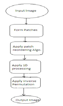
The technique explained in this paper introduces an image processing scheme based on reordering of its patches. For a given corrupted image, the image is divided into set of patches with overlaps and orders them by applying shortest possible path essentially solving travelling salesman problem. The result of ordering is applied to the corrupted image enabling good recovering of the image.
.
—————————— ——————————
n recent years as the use of images is increased so as techniques to Iprocess them. Let this processing be for removing noise or distortions from the image or changing some features of the image. Among these techniques the image processing using local patches has become very popular and was very effective. [1]-[13].All of them follow the core idea : given the image to be processed , extract all possible patches with over- laps; let the patch size be typically very small (a typical patch size would be 8 X 8 pixels ).The processing starts by operating on these patches and making use of interrelations in them.
There are various ways in which interrelations between patches can be used: NL-means algorithm, it takes weighted average of pixels with similar
surrounding patches [1], cluster the patches into disjoint sets and treat each set differently [2]-[7], seek a representative dictionary for patches and use it to sparse representation of them [8]-[11], form group of similar patches and apply a sparsifying transform on them [10],[12],[13].A com- mon thing in all of these methods is that every patch from image may find similar patch extracted elsewhere in the image. Thus believing that they form a high-structured geometrical form in the embedding space they reside in. If we treat these patches jointly, they support the reconstruction process by introducing a non-local force giving good recovery.
In the technique proposed here, all the patches with maximal overlaps are extracted. Their spatial relationship is disregarded and a complete new way for organizing them is found out. The patches are referred as cloud of vectors/points in proposed technique and they are chained in the shortest possible path essentially solving travelling salesman problem. The pro- posed method works on key assumption that proximity between two patches implies proximity between their center pixels, which helps to main- tain good quality of the image. W hen the image is deteriorated suppose due to noise or containing missing pixels the proposed method suggests a reordering of the corrupted pixels to what should be a regular signal. Thus we can have good recovery of the image by applying relatively simple one
dimensional smoothing operation.
The paper is organized into following sections: Section 2 provides an insight into related works carried out in the field of study; proposed work is highlighted in Section 3; working of the system is explained in the section
4. Methodology of the work is elaborated in Section 5. Experimental re- sults are discussed in Section 6 and finally Section 7 sums up the contri- bution in the current paper with concluding remarks.
2. AN INSIGHT INTO RELATED WORK Related Work
In image processing much work has been done in patch reordering
and various algorithms have been developed for the consideration of the pixels and then visiting nearby pixels. The working principle of all these algorithms is almost same like first extract all possible patches with over- laps; these patches are typically very small compared to the original image size (a typical patch size would be 8 X 8 pixels). The processing itself proceeds by operating on these patches and exploiting interrelations be- tween them. The manipulated patches (or sometimes only their center pixels) are then put back into the image canvas to form the resulting im- age. There are various ways in which the relations between patches can be taken into account they are explained as follows:
2.1 NL-Means algorithm [2]
In this method the basic working is kept as it is like converting image into patches and then any random pixel is taken into account to start with. Then the similar surrounding patches are considered and their weights are calculated from current considered pixel. This process is repeated for all the similar surrounding patches. Finally their average is calculated and then compared with threshold value and the ordering is decided accord- ingly.
Drawback - Causes performance issue for large images.
IJSER © 2014 http://www.ijser.org
International Journal of Scientific & Engineering Research, Volume 5, Issue 7, July-2014 1260
ISSN 2229-5518
2.3.2 Clustering of patches [3]
In this method the patches with similarities are grouped into so called clusters. These clusters are treated as disjoint sets and then each set is treated differently. The pixels of each cluster are considered and first the complete patch is processed and then the second disjoint set i.e. second cluster of patches is considered and so on till all the image patches are processed.
Drawback- complex in implementation.
2.3.3 Sparse representation of patches [4]
In this method the basic working is kept as it is like converting image into patches and then any random pixel is taken into account to start with. Then the similar surrounding patches are considered and their weights are calculated from current considered pixel. This process is repeated for all the similar surrounding patches. Finally their average is calculated and then compared with threshold value and the ordering is decided accord- ingly.
Drawback - Causes performance issue for large images.
2.3.4 Sparsifying global transform [5]
In this method after the image taken as set of patches, a different repre- sentation format is used. The patches are represented in the a representa- tive dictionary for the patches and then this representation format is used to sparsely represent them .Then this sparse representation gives then reordering structure.
A common theme to many of these methods is the expectation that every patch taken from the image may find similar ones extracted else- where in the image. The image patches are believed to exhibit a highly- structured geometrical form in the embedding space they reside in. A joint treatment of these patches supports the reconstruction process by intro- ducing a non-local force, thus enabling better recovery.
2.5 Patch based image processing approach
In this method an image-adaptive wavelet transform is constructed which is tailored to sparsely represent the given image. A plain 1D wavelet trans- form is used and adapted to the image by operating on a permuted order of the image pixels. The permutation is drawn from a shortest path order- ing of the image patches. This way, the patches are leveraged to form a multiscale sparsifying global transform for the image in question.
All the techniques explained here are having patch based approach for processing the image only how they process the patch is differentiates them from each other. Every method is having some advantages as well as disadvantages in accordance with the applications.
They can be compared and summarized as follows: Comparison of approaches:
The core process of the proposed approach is: for a given corrupted im- age, its pixels are reordered. Then operations are performed on the new
1D signal using simplified algorithms and the resulting values are reposi- tioned to their locations. Thus reordering the pixels and getting better im- age. The proposed approach is compared with two very popular algo- rithms K-SVD algorithm [8] for medium and high noise levels and BM3D algorithm for high noise levels and can see that the proposed approach works better than these two.
Basic steps:
1. Reading image
2. Building Permutation Matrix
3. Distance Measure between patches
4. Measuring Total Variance
5. Searching nearest Neighborhood patches
6. Reconstructing de noised output image
7. Calculating PSNR Value
8. Apply Distance Measure between patches with different Direc- tion.
IJSER © 2014 http://www.ijser.org
International Journal of Scientific & Engineering Research, Volume 5, Issue 7, July-2014 1261
ISSN 2229-5518
to handle. Our goal is to reconstruct y from z, and for this permutation matrix P of size N X N is employed. when P is applied to the target signal y, it produces a smooth signal yp = Py We start by applying P to z and obtain zp = Pz.and then apply a simple 1D smoothing operator H on zp ,
such as 1D interpolation or filtering. Finally, we apply P-1 to the result, and
obtain the reconstructed image^y = P-11HPz. In order to better smooth the recovered image, we use an approach which resembles the cycle spinning method. We randomly construct K different permutation matrices P k , uti- lize each to denoise the image z using the scheme described above, and average the results. This can be expressed by![]()
3.2 Algorithm of proposed approach
Task: Reorder the image patches x j,
Parameter: We are given the image patches {Xj } where j=1 to n,the distance function and" which is used in probabilistic part of the algorithm.
Fig: Algorithm of proposed system.
For forming patches pixels of very small area are considered. Initially the
√8 X √8 pixel patch is considered
Settles with values obtained from suboptimal ordering operation, using patches from the corrupted image. Values are entered by taking help of set O. The permutation matrix P is applied to input image to reorder the pixels.
Need Permutation matrix P was designed to reorder the signal composed of the middle points in the patches. n sub images are considered of size![]()
Where n is the patch size and N 1 X N 2 =N
And apply denoising transformations with averaging so that improved denoising results are obtained.
3.1 Mathematical model of proposed approach
Let Y be an image of size N1 X N2 where N1,N2 = N, and let Z be a cor- rupted version of Y, which may be noisy or contain missing pixels.
Also, let z and y be the column stacked versions of Z and Y, respectively. Then it is assumed that the corrupted image satisfies z = My + v(1) where the N X N matrix M denotes a linear operator which corrupts the data, and v denotes an additive white Gaussian noise independent of y with zero
mean and variance σ 2. In this work the matrix M is restricted to represent
a point wise operator, covering applications such as denoising and inpaint- ing. The reason for this restriction is the fact that we will be permuting the pixels in the image, and thus spatial operations become far more complex
Initialization: choose a random index j and set
Ω (1) = {j}
Main Iteration: Perform the following steps for k = 1…N-1
1. Set A k to be the set of indices of the B X B patches around
X Ω,k
2. Ak / Ω =1 then set Ω (k+1) to be A k /Ω
Else if
Else If A k >= 2
Find Xj1 the nearest neighbor to x Ωk such that j 1 ε A k and j1 not εA k . Find X j2 the second nearest neighbor to xΩk such that j 2 εAk and j2 not εA k .
Else if A k / Ω = = 0 Find x j1 - the nearest neighbor to xΩk such that j1 not εΩ
Find xj2 - the nearest neighbor to x k such that j2 notεΩ set Ω(k + 1) to
be : {j 1 } with probability P1 α exp[- ω(xΩk ,x j1) /ε]
{j2} with probability
P2 = 1 – P1 α exp[- ω(xΩk ,x j1) /ε]
Output : The set holds the proposed ordering.
We can visit patches in proposed approach the immediate pixels which are at the east, west,south and north directions are visited and the pro- cess is repeated till we visit all the pixels in the patches.
This can be represented mathematically as:
P1(e) α exp [- ω(x ji ; xi+1 )/ ε] P1(w) α exp [- ω(xji ; xij-1 )/ ε] P1(n) α exp [- ω(x ji ; xj+1,i )/ ε] P1(s) α exp [- ω(x ji ; x j,i-1 )/ ε]
IJSER © 2014 http://www.ijser.org
International Journal of Scientific & Engineering Research, Volume 5, Issue 7, July-2014 1262
ISSN 2229-5518
1. Take an image of size N.
2. Add some white Gaussian noise (mean =0, variance= sigma^2) in parallel.
3. Create a permutation matrix of size N that smoothens the distorted image in parallel.
4. Apply 1D smoothing operator (H) like 1D interpolation or filtering in
parallel.
5. Apply inverse of permutation matrix to get the reconstructed image.
6. Optimization:- repeat step 5 for k different permutation matrices, de- noise, and average the results. (May be in parallel)
Let xi be column stacked version of the √n x √n patch around the loca- tion of zi in Z.
A column stacked version of a matrix means that it's a column vector, which is created by concatenating the columns of this matrix one by one.
1. Find Euclidean_Distance (patch xi , patch x j)
A.Proximity between the two patches suggests the proximity be- tween the uncorrupted versions of their center pixels yi and yj B.Reorder the xi ’s to get smooth path
C.Apply total-variation measure to measure the smoothness of
the reordered signal
3) Shrinkage of the transform spectrum coefficients;
4) Inverse 3D transformation. This 3D filter therefore filters out simulta-
neously all 2D image patches in the 3D block.
We will perform the Perform image denoising using Non-local Means Denoising algorithm with some computational optimizations. Denoising of a color image u=(u1, u2, u3) and a certain patch B = B(p,f) (centered at p and size 2f+1 x 2f+1) writes
where i=1, 2, 3, B(p, r) indicates a neighborhood centered at p and size
2r+1 × 2r+1 pixels and w(B(p,f),B(q,f)) has the same formulation than in the pixelwise implementation.
In this way, by applying the procedure for all patches in the image, we shall dispose of N² = (2f+1)² possible estimates for each pixel. These es- timates can be finally averaged at each pixel location in order to build the final denoised image.
The main difference of both versions is the gain on PSNR by the
D.Apply Xp
points x p
measure for smoothness of the path through the
patchwise implementation, due to the larger noise reduction of the final aggregation process. Spurious noise oscillations near edges are also re-
2. Find the shortest path between set of points xi using nearest neigh- bor algorithm (may be in parallel) with suitable probabilities & surround- ing square neighborhood with BxB patches.
Extract the √n x √n image patches from the input image
1. Construct a matrix of size n x (N 1 - √n + 1) (N 2 - √n + 1) column stacked matrix of all the patches.
A.From left-most one, scan each patch column by column. B.Utilize the permutation matrix pixel associated with middle
pixel, constructed in module B.
C.Reorder any one of the signals located in the rows of column stacked version of a patch.
D.Apply inverse permutation on the result and obtain the recon- structed subimages.
E.Reconstruct the image from all the reconstructed subimages by suitable reordering and averaging the different values obtained for each pixel using the diagonal weight matrix.
F.Generate K random matrices and repeat the steps a-d.
Connection to BM3D:
Non-locality is a powerful recent paradigm in Image Processing that was introduced around 2005. Put in simple words, it consists in consider- ing that an “image is a collection of highly redundant patches”. In this con- text, pixels get described by the surrounding patch instead of their sole value), and patch relationships are only deduced from their visual similarity (thus ignoring their spatial relationship).
Non-locality comes in two flavors: exemplar-based or sparsity-based. The most famous example of sparsity based non-local algorithm is BM3D, and it is still considered as a top-ranking denoising algorithm. Collabora- tive filtering is the name of the BM3D grouping and filtering procedure. It is realized in four steps:
1) Finding the image patches similar to a given image patch and group- ing them in a 3D block
2) 3D linear transform of the 3D block;
duced by the final aggregation process. However, the overall quality in terms of preservation of details is not improved by the patchwise version.
PARAMETERS
The size of the patch and research window depend on the value of σ. When σ increases we need a larger patch to make patch comparison robust enough. At the same time, we need to increase the research win- dow size to increase the noise removal capacity of the algorithm by finding more similar pixels.
The value of the filtering parameter writes h= k σ. The value of k de- creases as the size of the patch increases. For larger sizes, the distance of two pure noise patches concentrates more around 2σ² and therefore a smaller value of k can be used for filtering.
Preprocessing:
1. Consider a diagonal matrix M of size NxN.
A.1 in principal diagonal correspond to existing pixels
B.0’s in principal diagonal correspond to missing pixels
2. Scan each patch to find the missing pixels.
A.Set Si as the indices to missing pixels in the diagonal matrix.
3. Find Euclidean Distance(patch xi , patch x j ) according to the formula
(20).
Algorithm:
1. Calculate the permutation matrix.
2. If there is no sharing of pixels with unvisited patches, choose the next patch to be its nearest spatial neighbor.
3. Apply the obtained matrix to the subimages & observer the permut- ed vectors containing missing values.
4. Apply the operator H (cubic interpolation) on subimages, to recover he missing values.
5. Apply inverse of permutation matrix on resulting vectors and obtain the estimated subimages.
6. Calculate the final estimate from these subimages using formula (7).
IJSER © 2014 http://www.ijser.org
International Journal of Scientific & Engineering Research, Volume 5, Issue 7, July-2014 1263
ISSN 2229-5518
7. Apply two additional iterations of steps 1-6.
8. Rebuild P using reconstructed subimages to obtain full patches. The results can be mentioned in the tabular form as :-
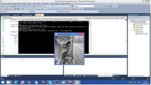
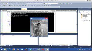
Following snapshots shows output for real time image taken from mo- bile and with real time noise. Hand shaked when taking image so image is blur. The three iteration output is displayed -
Following table shows Inpainting results (PSNR in db) of corrupted versions of the images of Lena,Barbara and House with 80 percents of their pixels missing obtained using triangle based cubic interpolation (tri. Cubic) over complete DCT dictionary 1 and 3 iterations of proposed scheme.For each image best result is hightlighted.
IJSER © 2014 http://www.ijser.org
International Journal of Scientific & Engineering Research, Volume 5, Issue 7, July-2014 1264
ISSN 2229-5518
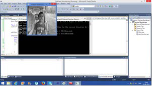
The PSNR values per iteration are :
A new image processing scheme is proposed here which is based on smooth 1D ordering of the pixels in the given image. Using a carefully designed permutation matrices and simple and intuitive 1D operations such as linear filtering and interpolation, the proposed scheme can be used for image denoising and inpainting, with better performance and results .
[1] Idan Ram, Michael Elad, Fellow, IEEE, and Israel Cohen, Senior Member, IEEE, ”Image Processing Using SmoothOrdering of its Patch- es”, IEEE transaction on image processing.vol. 22, No.. 7, JULY 2013
[2] A. Buades, B. Coll, and J. M. Morel, “A review of image denoising algorithms, with a new one,” Multiscale Model. Simul., vol. 4, no. 2,
pp. 490–530, 2006.[3] P. Chatterjee and P. Milanfar, “Clustering- based denoising with locally learned dictionaries,” IEEE Trans. Image Process., vol.
18, no. 7,pp. 1438–1451, Jul. 2009.
[4] G. Yu, G. Sapiro, and S. Mallat, “Image modeling and enhance- ment via structured sparse model selection,” in Proc. 17th IEEE Int. Conf. Image
Process., Sep. 2010, pp. 1641–1644.
[5] G. Yu, G. Sapiro, and S. Mallat, “Solving inverse problems with piecewise linear estimators: From Gaussian mixture models to structured
sparsity,” IEEE Trans. Image Process., vol. 21, no. 5, pp. 2481–2499, May 2012.
[6] W. Dong, X. Li, L. Zhang, and G. Shi, “Sparsity-based image de- noising via dictionary learning and structural clustering,” in Proc. IEEE Conf.
Comput. Vis. Pattern Recognit., Jun. 2011, pp. 457–464.
[7] W. Dong, L. Zhang, G. Shi, and X. Wu, “Image deblurring and superresolutionby adaptive sparse domain selection and adaptive regular- ization,”IEEE Trans. Image Process., vol. 20, no. 7, pp. 1838–1857,Jul.
2011.
[8] D. Zoran and Y. Weiss, “From learning models of natural image patches to whole image restoration,” in Proc. IEEE Int. Conf. Comput. Vis.,
Nov. 2011, pp. 479–486.
[9] M. Elad and M. Aharon, “Image denoising via sparse and redun- dant representations over learned dictionaries,” IEEE Trans. Image Pro- cess.,
vol. 15, no. 12, pp. 3736–3745, Dec. 2006.
[10] J. Mairal, M. Elad, and G. Sapiro, “Sparse representation for color image restoration,” IEEE Trans. Image Process., vol. 17, no. 1, pp. 53–69,
Jan. 2008.
[11] J. Mairal, F. Bach, J. Ponce, G. Sapiro, and A. Zisserman, “Non- local sparse models for image restoration,” in Proc. IEEE 12th Int. Conf.
Comput. Vis., Sep.–Oct. 2009, pp. 2272–2279.
[12] R. Zeyde, M. Elad, and M. Protter, “On single image scale-up us- ing sparse-representations,” in Proc. 7th Int. Conf. Curves Surf., 2012,
pp. 711–730.
[13] K. Dabov, A. Foi, V. Katkovnik, and K. Egiazarian, “Image de- noising by sparse 3-D transform-domain collaborative filtering,” IEEE Trans.
16, no. 8, pp. 2080–2095, Aug. 2007.
[14] X. Li, “Patch-based image interpolation: Algorithms and applica- tions,” in Proc. Int. Workshop Local Non-Local Approx. Image Process.,
2008,
IJSER © 2014 http://www.ijser.org
pp. 1–6.
International Journal of Scientific & Engineering Research, Volume 5, Issue 7, July-2014 1265
ISSN 2229-5518
[15] I. Ram, M. Elad, and I. Cohen, “Generalized tree-based wavelet transform,”IEEE Trans. Signal Process., vol. 59, no. 9, pp. 4199–4209,
Sep. 2011.
[16] I. Ram, M. Elad, and I. Cohen, “Redundant wavelets on graphs and high dimensional data clouds,” IEEE Signal Processing Letters, vol.
19,
no. 5, pp. 291–294, May 2012.2774 IEEE TRANSACTIONS ON IM- AGE PROCESSING, VOL. 22, NO. 7, JULY 2013
[17] G. Plonka, “The easy path wavelet transform: A new adaptive wavelet transform for sparse representation of two-dimensional data,” Multiscale
, no. 3, pp. 1474–1496, 2009.
[18] D. Heinen and G. Plonka, “Wavelet shrinkage on paths for de- noising of scattered data,” Results Math., vol. 62, nos. 3–4, pp. 337–354,
2012.
[19] T. H. Cormen, Introduction to Algorithms. Cambridge, MA, USA: MIT Press, 2001.
[20] M. Elad, Sparse and Redundant Representations: From Theory to Applications in Signal and Image Processing. New York, NY, USA:
Springer-Verlag, 2010.
[21] R. R. Coifman and D. L. Donoho, “Translation-invariant de- noising,” Wavelets and Statistics. New York, NY, USA: Springer-Verlag,
1995,
pp. 125–150.
[22] T. Yang, Finite Element Structural Analysis, vol. 2. Englewood
Cliffs, NJ, USA: Prentice-Hall, 1986.
[23] D. Watson, Contouring: A Guide to the Analysis and Display of
Spatial Data (With Programs on Diskette). New York, NY, USA: Pergamon,
1992.
IJSER © 2014 http://www.ijser.org