would seem to be permit. (Bronshtein et al.,1985)
International Journal of Scientific & Engineering Research, Volume 4, Issue 12, December-2013 134
ISSN 2229-5518
Probability and Statistics
Anam Saghir (2013)
Abstract:Probability and statistics are two different confusing tools in genetics.They create inexactness not only for the geneticist but also for the biologist as the genetics is the leading field in biology.So this paper discusses the basic tools interpreting probability and genetics and answers the questions regarding to chance event in probability with different rules,formulas and experiments while its chi-square test explain the degree of freedom with related experiment. So, it represents adequate factual analysis and findings,which will help all researchers,students of genetics to clear their concept.
results are evidence of the existence of some mechanism
,which allowed the subject to perform better than chance
Probability and statistics are two different
confusing tools in genetics.They create inexactness not only for the geneticist but also for the biologist as the genetics is the leading field in biology.So this paper discusses the basic tools interpreting probability and genetics and answers the questions regarding to chance event in probability with different rules,formulas and experiments while its chi- square test explain the degree of freedom with related experiment. So, it represents adequate factual analysis and findings,which will help all researchers,students of genetics to clear their concept.In the scientific method, scientists make predictions, perform investigation, and gather data that they then compare with their original predictions. The problem is that we live in a world permeated by random and stochastic events. (Abramowitz et,al.,1974)
We need probability theory to tell what to expect from the data.Most experimental searches for telegnostic phenomena are statistical in nature. A subject repeatedly attempts a task with a known probability of success due to chance, then the number of actual successes is compared to the chance and the expectation. If a subject scores consistently higher or lower than the chance expectation after a large number of assays, one can calculate the probability of such a score due to pure chance and then argue, if the chance probability is sufficiently little, that the
would seem to be permit. (Bronshtein et al.,1985)
Suppose you ask a question to guess, before it is flipped, whether a coin will land with heads or tails up. Assuming the coin is fair (has the same probability of heads and tails) the chance of guessing correctly is 50%, so you'd expect half the guesses to be correct and half can be wrong. So, if we ask the subject to guess heads or tails for each of
100 coin flips, we would expect about 50 of the guesses can be correct. Suppose a new subject introduces into the lab and manages to guess heads or tails correctly for 60 out of
100 tosses. Evidence of precognition or perhaps the subject's possessing a telekinetic power which causes the coin to land with the guessed face up, Well you can not say that. In all likelihood , we have observed nothing more than good luck. The probability of 60 right guesses out of 100 is
IJSER © 2013 http://www.ijser.org
International Journal of Scientific & Engineering Research, Volume 4, Issue 12, December-2013 135
ISSN 2229-5518
about 2.8%, which means that if we do a large number of experiments flipping 100 coins, about every 35 experiments
we can expect a score of 60 or better, purely due to chance of expression. (Graham et al., 1998)
When events are mutually pronominal , the sum rule is used.The probability that one of several mutually prenominal events will occur is the sum of the probabilities of the individual events.This is also known as the either-or
that number of heads can occur, divided by the number of total after-effects of four flips are 16. We can then tabulate
the probabilities as under
Number of Heads | Number of Ways | Probability |
0 | 1 | 1/16 = 0.0625 |
1 | 4 | 4/16 = 0.25 |
2 | 6 | 6/16 = 0.375 |
3 | 4 | 4/16 = 0.25 |
4 | 1 | 1/16 = 0.0625 |
![]()
Example:
Since we are absolutely certain the number of heads we get in four flips is going to be between zero and four, the probabilities of the difference in numbers of heads should
For example, the chance of rolling either a 2 or a 3 on a die will be
P = 1/6 + 1/6 = 2/6 = 1/3( Hogben et al.,1937)
When the occurrence of one event is independent of the occurrence of other events, the product rules are used.This is known as the and rule.
Since the coin is fair, each flip has an similar chance of coming up heads or tails, so all 16 possible outcomes tabulated above are equally presumptive. But since there are 6 ways to get 2 heads, in four flips the probability of two heads is more than that of any other result. We will express probability as a number between 0 and 1. A probability of zero is a result which cannot ever occur, the probability of getting five heads in four flips is zero. A probability of one represents certitude, if you flip a coin, the probability you will get heads or tails is one (assuming it can notland on the rim, fall into a black hole, or some such).The probability of getting a given number of heads from four flips is, then, simply the number of ways
sum up to 1. Adding the probabilities in the table confirms
it. Further, we can calculate the probability of any collection
of results by summing the individual probabilities of each number. Suppose we would like to know the probability of getting lesser than the three heads from four flips. There are three ways this can happen: zero, one, or two heads.
The probability of lesser than three, then, is the sum of the probabilities of all these results, 1/16 + 4/16 +
6/16 = 11/16 = 0.6875, or a little more than two out of all three. So we can calculate the probability of one outcome or another, sum or add the probabilities.
To get probability of one result and another from two separates the experiments, multiply the individual probabilities. The probability of getting a head in 4 flips is
4/16 = 1/4 = 0.25. What is the probability of getting one head
in each of two consecutive sets of four flips? Well, it is just
1/4 × 1/4 = 1/16 = 0.0625.
The probability for any number of heads x in any number of flips n is thus the number of ways in which x heads can occur in n flips,
IJSER © 2013 http://www.ijser.org
International Journal of Scientific & Engineering Research, Volume 4, Issue 12, December-2013 136
ISSN 2229-5518
2. The coefficients in front of these terms: 1,
2, and 1, are the number of various
families of the given type.Thus there are 2 different families with 1 normal and 1 mutant child, normal born first and mutant born second, or mutant born first and normal born latter on.
divided by the number of different possible results of flips, calculated by number of heads. But there is no need to add the combinations in the denominator, since the number of possible results is simply two increased to the power of the number of flips. So, we can elaborate the expression for the probability to:
As before, p = 3/4 and q = 1/4.Chance of 2 normal children =
p2 = (3/4)2 = 9/16.
Chance of 1 normal plus 1 mutant = 2pq = 2 * 3/4 * 1/4 =
6/16 = 3/8.
p 2 + 2 pq + q 2
(Knuth et al,.
Here, p3 is a family of 3 normal children, 3p2q is 2
normal plus 1 affected, 3pq2 is 1 normal plus 2 affected,
IJSER
![]()
Binomial Theorem:
1997)
and q3 is 3 affected children. The exponents on the p and q represent the number of children of each form.The
The binomial theorem is used for disordered events.The probability that some arrangement will occur in which the final order is not qualified is defined by the binomial theorem.![]()
For Larger Families:
1. The main method of all accomplishable families
coefficients are the number of families of this type.
Chance of 2 normal + 1 affected is explained by the term
3p2q. Thus, 3 * (3/4)2 * 1/4 = 27/64. Same as we got by
enumerating the families in a list. (Montgomery et al.,1994)
and counting the ones of the proper type gets bunglesome with big families.
2. The binomial distribution is a small method based
on the expansion of the equation to the right,
p3 + 3 p2 q + 3 pq2
+ q3 = 1
where p = probability of one event (say, a normal child), and q = probability of the alternative event
9mutant child). n is the number of children in the family.
3. Since one raised to any power (multiplied by itself) is always equal to 1, this equation describes the probability of any size of family. (Press et al,.1992)
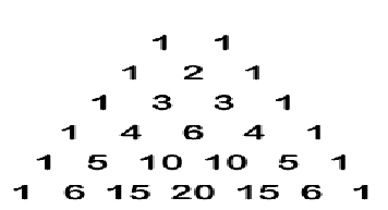
Pascal’s Triangle is a way of finding the coefficients for the binomial in a undecomposable way.Start by writing the coefficients for n = 1: 1 1.Below this, the coefficients for n = 2 are found by putting 1 on the outside and adding up adjacent coefficients from the line above as
1, 1 + 1 = 2, 1.Next line will be in the same way,write 1’s on
the outsides, then sum up adjacent coefficients from the line
( p +
q) n = 1
above,1, 1+2 = 3, 2+1 = 3, 1.For n = 5, coefficients will be 1, 5,
10, 10, 5, 1.( Huff &Darrell ,1993)
1. The expansion of the binomial for n = 2 is shown. The 3 terms represent the 3 different kinds of families, p2 is families with 2 normal children, 2pq is the families with 1 normal and 1 mutant child, and q2 is the families with 2 mutant children.
IJSER © 2013 http://www.ijser.org
International Journal of Scientific & Engineering Research, Volume 4, Issue 12, December-2013 137
ISSN 2229-5518
A method of statistics used to know goodness of fit.Goodness of fit refers to how close the observed data are to those prognosticate from a hypothesis.The general formula is
assumed that chance alone produced the difference. Conversely, when the
probability is less, it is thought that a significant value other than it will deviate.
– In 1912, Arthur Harris applied Pearson's chi-square test to examine Mendelian ratios (Harris, 1912). It is essential to note that when Gregor Mendel studied inheritance, he did not use statistics and neither did Bateson, Saunders, Punnett, and Morgan during the experiments that discovered genetics linkage. Thus, until Pearson's statistical tests were applied to biological data, scientists judged the goodness of fit between expected and observed experimental results simply by inspecting the data and drawing conclusions (Harris,
1912). Although this method can work
perfectly if one's data exactly pairs one's predictions, scientific experiments often have variability related with them, and
this makes statistical tests very utilizable.
– The chi-square value is calculated using
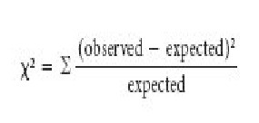
(O-E)2 /E
the following formula:
where
– O = observed data in each category
– E = observed data in each category based on the experimenter’s hypothesis
– S = Sum of the calculations for each
category
– One of Pearson's most
momentous achievements occurred in
1900, when he developed a statistical
test called Pearson's chi-square (Χ2) test,
also known as the chi-square test for the goodness of fit (Pearson, 1900). Pearson's chi-square test is used to check the role of chance in producing deviations between observed and expected values. The test depends on an adventitious hypothesis, because it requires theoretical values to be calculated,which are expected. The test indicates the probability that chance alone produced the deviation between the expected and the observed values.When the probability calculated from Pearson's chi-square test is more, it is
Using this formula, the change between the actual and theoratical frequencies is calculated for each experimental result category. The difference is then squared and divided by the expected frequency. Finally, the chi- square values for each outcome are added together, as represented by the summation sign (Σ).
Pearson's chi-square test works good with genetic data as long as there are sufficient expected values in each group. In this case of little samples (less than 10 in any category) that have 1 degree of freedom, the test is not certain. (Degrees of freedom, or df, will be explained in full later in this article.) However, the test can be corrected by using the Yates correction for continuity, which reduces the direct value of each difference between observed and expected frequencies by 0.5 before squaring. Additionally, it is important to remember that the chi-square test can only
IJSER © 2013 http://www.ijser.org
International Journal of Scientific & Engineering Research, Volume 4, Issue 12, December-2013 138
ISSN 2229-5518
be applied to numbers of progeny, not to harmonises or
percentages.
Now that you know the rules for using the test, it is time to chew over an example of how to calculate Pearson's chi-square. Recall that when Mendel crossed his pea plants, he learned that tall (T) was dominant to recessive (t). You want to confirm that this is right, so you start by formulating the following null hypothesis,In a cross between two heterozygote (Tt) plants, the offspring should occur in a 3:1 ratio of tall plants and short plants. Next, you pass over the plants, and after the cross, you measure the properties of 400 offspring. You note that there are 305 tall pea plants and 95 short pea plants, these are your experimental values. Meanwhile, you expect that there will be 300 tall plants and 100 short plants from the Mendelian ratios.
You are now ready to perform statistical analysis of your results, but first, you have to choose a faultfinding value at which to reject your null hypothesis. You opt for a
critical value probability of 0.01 (1%) that the deviation
The add up of the two categories is 0.08 + 0.25 =
0.33Therefore, the overall Pearson's chi-square for the
experiment will be Χ2 = 0.33
Next, you will determine the probability that is affiliated with your calculated chi-square value. To do this, you compare your calculated chi-square value with theoretical values in a chi-square table that has the same number of degrees of freedom. Degree of freedom shows the number of ways in which the observed outcome categories are free to change. For Pearson's chi-square test, the degrees of freedom are equal to n - 1, where n shows the number of different theoretical phenotypes (Pierce,
2005). In your experiment, there are two expected
outcome phenotypes, so n = 2 categories and the degrees of
freedom equal 2 - 1 = 1. (Sham,1998)
1. Abramowitz, Milton and Irene A.
Stegun. Handbook of Mathematical
Functions (Chapter 26). New York: Dover, 1974.
IJSER
between the observed and expected values is due to chance
event. This means that if the probability is less than 0.01,
then the deviation is significant and it is not due to chance
and you will reject your null hypothesis. However, if the deviation is greater than 0.01, then the deviation is not significant and you will not reject the null hypothesis.So, should you reject the null hypothesis or not! Here is a summary of your observed and expected data.
Tall | Short | |
Expected | 300 | 100 |
Observed | 305 | 95 |
Table 2:Data for Statistical Analysis
Now, let's calculate Pearson's chi-square: For tall plants: Χ2 = (305 - 300)2 / 300 = 0.08
For short plants: Χ2 = (95 - 100)2 / 100 = 0.25
ISBN 0-486-61272-4.
2. Bronshtein, I.N. and K.A.
Semendyayev. Handbook of Mathematics (Chapter
5). Frankfurt/Main: Verlag Harri Deutsch, 1985. ISBN 0-442-21171-6.
3. Hogben, Lancelot. Mathematics for the
Million (Chapter 12). New York: W.W. Norton,
1937, 1967. ISBN 0-393-30035-8.
4. Graham, Ronald L., Donald E. Knuth, and Oren Patashnik. Concrete Mathematics: a Foundation for Computer Science (Chapter 8). Reading, Massachusetts: Addison-Wesley, 1988. ISBN 0-201-
14236-8.
5. Knuth, Donald E. The Art of Computer Programming, Volume 2, Seminumerical Algorithms (Third Edition) (Chapter 3). Reading, Massachusetts: Addison-Wesley, 1997. ISBN 0-201-
89684-2.
6. Press, William H., Saul A. Teukolsky, William T.
Vetterling, and Brian P. Flannery. Numerical
Recipes in C (Second Edition) (Chapter 14). Cambridge, England: Cambridge University Press,
1992. ISBN 0-521-43720-2.
7. Montgomery, Douglas C. and George C.
Runger. Applied Statistics and Probability for
Engineers . New York: John Wiley & Sons, 1994. ISBN 0-470-09940-2.
8. Huff, Darrell. How to Lie with Statistics . New
York: W.W. Norton, 1993. ISBN 0-393-31072-8.
IJSER © 2013 http://www.ijser.org
International Journal of Scientific & Engineering Research, Volume 4, Issue 12, December-2013 139
ISSN 2229-5518
9. Pearson, K. On the criterion that a given system of deviations from the probable in the case of
correlated system of variables is such that it can be reasonably supposed to have arisen from random sampling. Philosophical Magazine 50, 157–175 (1900)
10. Harris, J. A. A simple test of the goodness of fit of
Mendelian ratios. American Naturalist 46, 741–745 (1912)
11. Pierce, B. Genetics: A Conceptual Approach (New
York, Freeman, 2005)
12. Sham P (1998) Statistics in human genetics. Arnold
publishers
Author Details:Anam Saghir
,BS(hons.)7th,Zoology.Student at UOG Gujrat,Hafiz Hayat Campus,Pakistan(2013)
IJSER
IJSER © 2013 http://www.ijser.org