International Journal of Scientific & Engineering Research, Volume 5, Issue 4, April-2014 1
ISSN 2229-5518
Priority Assignment Based On Patronage Value
Uche, P. I and Ugah, T. E.
Department of Statistics, Faculty of Physical Sciences, University of Nigeria, ugahejiofor@yahoo.com
say x monetary units to the operator. In addition, he pays y monetary units as a processing fee (i.e. delivery charge). Based on sum of these
costs, herein called patronage value, the customer is commensurately placed in the queue. By buying more of the product and hence paying more money, the customer secures a position in the queue that shortens his stay in the system. Assuming, Poisson arrivals, exponential service time distribution and arbitrary distribution of customer payments, we obtain the expected number of customers in the system as a function of their payments and the system parameters. Also, an economic model is constructed and a closed-form expression of the economic cost service rate is obtained. An illustrating example based on Poisson arrivals, exponential service time distribution and lognormal distribution of payment is demonstrated.
Delay is an important consideration of efficiency when an organization sells a product to her customers, especially in situations where the time customers spend waiting for the service is an important factor apart from price that determines whether customers will do business with the organization. Afèche and Haim (2004) [2] observed that delay is a key dimension of service quality, playing an important role whenever a capacity-constrained provider faces delay-sensitive customers. When a queue is formed, customers lose valuable time and service-oriented organizations lose valuable customers via reneging and balking. Queues generate stress, cause and aggravate mistakes in addition to cost incurred by both the waiting customers and the facility operator. Thus, in a situation like this, the common economic theory that lowering the price increases the demand may be violated, since it is reasonable to expect customers to balk or renege when they anticipate a delay even when the price is lower.
Managing waiting lines creates a great of splitting
headache for managers seeking to improve the return on investment. If the waiting time and service time are high, customers may renege or balk thereby resulting in customer dissatisfaction. This will reduce customer demands and eventually the revenue.
Several administrative measures have been employed in regulating the arrival rate to a queuing system. One of them is priority pricing. Priority pricing has been studied in the context of queuing service facilities. Kleinrock (1967) [8] was the first to study the regulation of arrival process in a queue by a decentralized self-regulating mechanism that borders on bribing mechanism. He studied the allocation of priorities based on payments (bribe) made by customers. In Kleinrock's model, a new arrival offers a nonnegative payment, which he called
“bribe” to the queue manager. This customer is then assigned a position in the queue such that all those customers who made larger payments are in front of him and all those customers who made smaller payments are behind him. He derived steady-state expected waiting time as a function of their bribe.
Adiri and Yechiali(1977) [1] considered a service
station(facility) consisting of M separate priority queues. The higher the priority of the queue, the higher the priority price to join it, but the shorter the waiting time spent in the system. They derive the maximum profit price to be charged for joining each of the M separate priority queues.
Hanna (1988) [6] considered a profit making service facility that offers a set of different prices for the single service it provides. Interest is to determine the optimal number of priority classes and the set of prices that affords the service facility higher revenue than any other set. By paying a higher price, the customer buys into a priority class that shortens his stay in the service system. Balachandran (1972) [3] assumes that the customers are identical, and that they know the statistical distribution of the amounts other customers already in the system paid as well as the state of congestion of the system. He determined the best prices to be paid by customers on arrival for a system with an infinite number of classes where only one or two customers are allowed in each class.
In many service-oriented systems, arriving customers are not served on first- come-first-served basis, but according to a priority plan that ranks them with respect to their relative importance. It may not, however, an easy task to determine the importance level of customers, especially when such a decision needs to be made under scanty information about the customer. Such
IJSER © 2014 http://www.ijser.org
International Journal of Scientific & Engineering Research, Volume 5, Issue 4, April-2014 2
ISSN 2229-5518
systems aim to give priority to their delay-sensitive customers as well, as to make additional earnings from
N ( x, y ) =
![]()
{ρ 1 − F ( x)1 − F (y)}
2
such prioritization scheme. In this work we propose a prioritization scheme that ranks customers based on their patronage value. Under this arrangement, an arriving customer who pays x monetary units for the product
and y monetary units as a processing charge (i.e.
{1 − ρ 1- F ( x)1 − G( y)}
![]()
+ ρ 1 − F ( x)1 − F (y) (1)
{1 − ρ 1- F ( x)1 − G( y)}
delivery fee) is commensurately placed in the queue.
Consider an arriving customer whose pay x monetary
y
That is, based on the sum of these payments, the cost of
unit for the product and
monetary unit as a processing
the product x and the processing fee y the customer is placed appropriately in position on the queue. Thus, under this setting, a profit-making service facility, like a
manufacturing firm, can make its earnings from
customers' payments for the product it sells, in addition to extra earnings derivable from complementary service
such as the delivery of the product.
fee. This arriving customer has to wait for the following
before he leaves the system:
(i).He must wait until all the customers in the system before his arrival and whose payments are at least as big as his are served. The conditional arrival rate of customers whose payments lie in the region
{( z, z + dz ) ( u, u + du )}
and whose cost of product
and processing charge are least as big as x and y ,
respectively is
A queuing system whose prioritization criterion is based
∞ ∞ dF (u ) dG ( z )
![]()
λ dz du
( 2)
on the aforementioned arrangement is considered. The
case considered is that in which: (a) customers arrive
according to a Poisson process at a mean rate of λ customers per unit time. (b) The service time follows an exponential distribution with a mean service time 1![]() µ .
µ .
F ( x ) and G ( y )
∫∫ du dz
x y
By Little’s’ law (see [11], which states that the expected number of customers in the system is equal to the product of their arrival rate and the expected time they spend in the system, the expected total number of such customers in the system is
(c)We let
are the distribution functions
of X and Y , respectively. (e) The arrival time, the service
∞ ∞ dF (u ) dG ( z )
![]()
∫∫ λ W (u , z ) dz du
(3)
time and the payments are all independent random
x y
du dz
variables for each customer.me that (f). We also assume that X and Y are independent.
The mechanics of the system are as follow: Consider
an arrival to the system whose sum of payments is
Each of these customers causes him to wait an average of
1![]() µ units of time so that his expected waiting time for
µ units of time so that his expected waiting time for
them is
( x + y )
∞ ∞ λ dF (u ) dG ( z )
![]()
![]()
∫∫ W (u , z ) dz du
(4)
. This customer is placed in position on the
x y µ
du dz
queue so that all those customers whose sum of payments
( x + y ) > ( x + y )′
are behind him and all those whose sum
( x + y ) ≤ ( x + y )′′
(ii). The customer must wait until all the customers who come while he is still in the queue and whose payments exceed his are served. The expected number of
of payments
are in his front of him. An
W ( x, y )
these customers during his average wait is
arriving customer neither knows the actual number of
customers in front of him nor the actual amounts paid
∞ ∞ dF (u ) dG ( z )
W ( x, y ) ∫∫ λ dz du
(5)
they paid before making his payments. Instead, he knows the statistical distribution of the queue length and the amounts paid by other customers already in the queue.![]()
du dz
Similarly, each of these customers causes him to wait, on![]()
1 µ
W ( x, y )
the average,
units of time. Thus, his expected
We let
N ( x, y )
be the average waiting time and
waiting time for them is
∞ ∞ λ dF (u ) dG ( z )
the expected number of customers in the system.![]()
W ( x, y ) ∫∫
![]()
dz du (6)
Theorem.
Given the above assumptions of the model, the expected number of customers in the system is given by
x y µ
du dz
IJSER © 2014 http://www.ijser.org
International Journal of Scientific & Engineering Research, Volume 5, Issue 4, April-2014 3
ISSN 2229-5518
(iii).This customer’s expected service time is service time is
1![]() µ (7 )
µ (7 )
due to the assumption of the exponential distribution for the service time.
To obtain this customer’s expected waiting time in the system W ( x, y ) , we add up (4), (6) and (7) to get
of the cost model, use is made of the mean cost associated with the waiting of customers (called expected waiting cost) and the mean cost associated with the operation of the facility (called expected facility cost) and the performance measures of the queuing system that generates these costs.
The expected waiting cost per unit time, denoted by
W ( x, y )
∞ ∞
![]()
= ∫∫
λ dF (u ) dG ( z )
![]()
W (u , z ) dz du
E(WC) ,can be obtained as the product of cost of waiting
x y µ
du dz
∞ ∞
per unit time per customer, denoted by Cs
and the mean
+ W ( x, y )
λ dF (u ) dG ( z ) 1
![]()
![]()
![]()
∫∫ dz du +
(8)
x y µ
du dz µ
number of customers in the queue, denoted b. That is,
To obtain the expected number of customers in the system N ( x, y ) , we take advantage of the universal
validity of the Little’s’ law (see [10] and (2) to obtain
E(WC) = Cs N ( x, y ) (10)
Using (1), we have
{ρ [1 − F ( x)][1 − F (y)]}2
![]()
{1 − ρ [1- F ( x)][1 − G( y)]}2
E(WC) = Cs
(11)
∞ ∞
+ ρ [1 − F ( x)][1 − F (y)]
λ 1 − F ( x)1 − G( y)
λ dF (u ) dG ( z )
![]()

W (u , z ) dz du
∫∫
{1 − ρ [1- F ( x)][1 − G( y)]}
![]()
= x y
du dz
N ( x, y )
{1 − ρ 1- F ( x)1 − G( y)}
![]()
+ ρ 1- F ( x)1 − G( y) (9)
{1 − ρ 1- F ( x)1 − G( y)}
The expected facility cost per unit time, denoted by
E(FC) , can be obtained as the product of cost of serving
By Conservation law as Kleinrock (1965 ) [9], (9) gives (1).
With increasing emphasis on cost-effectiveness, facility managers need appropriate statistical guidelines based on
one customer, denoted by C f
E(FC) = C f µ
and the service rate µ , or
(12)
sound economic theory to aid them in providing quality service to customers at a convenient (minimum) cost. In view of this, in the queuing literature there exists an emerging tendency to study economic models in the
context of queuing service facilities. Some reasonable
The expected total cost per unit time, denoted by E(TC) is the sum of the expected facility cost E(FC) and expected waiting cost E(WC) . Adding equations (11) and (12), we have
{ρ [1 − F ( x)][1 − F (y)]}2
![]()
work has been done in the area of cost analysis of
E(TC) = C
{1 − ρ [1- F ( x)][1 − G( y)]}2
+ C µ (13)
s f
queuing systems as evident in works of Brigham (1955)
+ ρ [1 − F ( x)][1 − F (y)]
{1 − ρ [1- F ( x)][1 − G( y)]}
[4], Grassmann (1979) [5], Hillier (1963) [8], and Morse
(1958) [11].
In this section, we formulate a cost model to determine the optimal service rate µ .In the formulation
IJSER © 2014 http://www.ijser.org
International Journal of Scientific & Engineering Research, Volume 5, Issue 4, April-2014 4
ISSN 2229-5518
Our objective here is therefore to derive a computationally closed-form expression of the service rate µ that minimizes the expected total cost. We shall
make use of the fact that the waiting cost and the service rate are inversely related. Increasing the level of service capacity causes a decrease in both the queue length and waiting time. This action will result to a decrease in this cost component (waiting cost). However, increasing the level of service capacity or service facility capacity will result to an increase in the facility cost. That is, increasing
the service rate µ will result in less time spent by the
customer’s waiting and thus a lower waiting, but a higher service cost. Since increasing the capacity will result in a reduction in the waiting cost and an increase in the
φ = −Cs (3C f λ 1 − F ( x ) 1 − F ( y ) )
3
− 3(Cs C f λ 1 − F ( x ) 1 − F ( y ) )
ϕ =
+ C 2 3C λ 1 − F ( x ) 1 − F ( y ) )
Suppose that a queuing system of a service facility operates according to our proposed model with a single server, an
exponential inter-arrival time distribution with mean of eight minutes and exponential service time distribution. Furthermore, the cost of waiting is $0.10 per minute per customer and the facility cost is $0.165 per customer. We consider a preemptive system with lognormal distributed
payments.From above, λ = 0.125, Cs = $0.1,
facility cost, an appropriate decision to consider is to adjust the service capacity so that the sum of these costs,
C f = $0.165 . For each value of
1 − F ( x ) 1 − F ( x )
the expected total system cost is reduced to a convenient level. The minimum cost service rate may be found by differentiating the expected total facility cost with respect to µ , setting the derivative equal to zero, and solving
for µ . Thus, differentiating (13) and solving for µ , we obtain
µ | 0.126 | 0.15 | 0.342 | 0.366 | 0.39 | 0.414 |
E(WC) | 0.3995 | 0.2149 | 0.0373 | 0.0336 | 0.0305 | 0.028 |
E(FC) | 0.0208 | 0.0248 | 0.0564 | 0.0604 | 0.0644 | 0.0683 |
E(TC) | 0.4203 | 0.2396 | 0.0938 | 0.094 | 0.0949 | 0.0963 |
λC 1 − F ( x ) 1 − F ( y )
µˆ = λ 1 − F ( x ) 1 − F ( y ) −
and for λ < µ , we use a grid-search approach to obtain
the optimal value of the service rate using (13) and then compare it with the optimal value of the service rate obtained by using (14). For instance, if
1 − F ( x ) 1 − F ( x ) = 0.6143 , we use equation (13) and
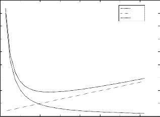
obtain the optimal value of the service rate µ which is shown in bold character in Table 1. Fig. 1 below is obtained by using the values in Table 1. It shows the relationship among the cost components and the service rate. It is typical of cost curves associate with waiting-line problems.
Table 1: Calculation of the Expected Costs![]()
1
[φ + ϕ ]3
1 1
33 [φ + ϕ ]3
(14)
−
where![]()
2
33 C f
IJSER © 2014 http://www.ijser.org
International Journal of Scientific & Engineering Research, Volume 5, Issue 4, April-2014 5
ISSN 2229-5518
0.45
0.4
0.35
0.3
0.25
0.2
0.15
0.1
E(WC) E(FC) E(TC)
[3] Balachandran,K.R(1972)., “ Purchasing Priorities in
Queues”, Management Science 18(5), pp.319-326.
[4] Brigham Georges (1955), “On a Congestion Problem in an Aircraft Factory”, Journal of the Operations Research Society of America, Vol. 3, No. 4,pp. 412-428
[5] Grassmann W. K. (1979) “ The Economic Service
Rate”, The Journal of the Operational Research Society, Vol.
30, No. 2. pp. 149-155
0.05
0
0.1 0.2 0.3 0.4 0.5 0.6 0.7 0.8 0.9
Level of Service
Figure1 Cost Curve
[6] Hanna Alperstein(1988), “.Optimal Pricing Policy for the Service Facility Offering a Set of Priority Prices”, Management Science 34(7), pp. 666–671.
[7] Hillier F.S. (1963), “The Application of Waiting-line
The minimum cost service rate µˆ
may also be obtained
Theory to Industrial Problems” J. Industrial Engineering,
15:3.
directly by substituting into equation (14) to obtain
µˆ = 0.342 customer per minute.
6 CONCLUSION
(15)
[8] Kleinrock, L. (1967), “Optimum Bribing for Queue
Position”, Oper. Res.,15 304–318.
[9] .Kleinrock, L.(1965), “A Conservation Law for a Wide
We proposed a simple and novel model for congestion alleviation that does not require stringent information about the customer. Based on the admission mechanism of the service facility, we derived the expected number of customers in the system. Also, we have also carried out an economic analysis of the system. A compact and computationally expression of the economic service rate that minimizes the expected total cost of service was also derived. The value of the service rate obtained by a grid- search approach and that obtained by direct substitution were observed to be the same. This model finds its application in manufacturing firms.
References
[1] Adiri,I and Yechiali,U(1974),”Optimal Priority- Purchasing and Pricing Decisions in Non-Monopoly and Monopoly Queues,” Oper. Res.,Vol.22 pp.1051-1066
[2] Afèche Philipp and Mendelson Haim,” Pricing and Priority Auctions in Queuing Systems”, Management Science 50(7), pp. 869–882.
Class of Queuing Disciplines”, Naval Res. Log. Quart.12:181-192.
[10] Little John D. C. (1960),” A Proof for the Queuing Formula: L = λW ” Case Institute of Technology, Cleveland, Ohio
[11] Morse, P.M (1958),” Queues, inventories and
Maintenance”, John Wiley and sons. New York.
IJSER © 2014 http://www.ijser.org