International Journal of Scientific & Engineering Research, Volume 4, Issue 7, July-2013 96
ISSN 2229-5518
Performance and Evaluation of Interferometric based Wavefront Sensors
M.Mohamed Ismail1, M.Mohamed Sathik2
Research Department of Computer Science, Sadakathullah Appa College (Autonomous), Tirunelveli -11, Tamilnadu, India
Email: mohammedismi@gmail.com
Email: mmdsadiq@gmail.com
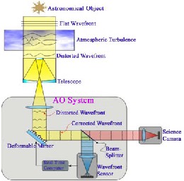
Atmospheric turbulence is the main cause of image degradation and poor resolution at the focal plane of a perfectly made optical telescope. It is necessary to make corrective measures to improve the optical wavefront, thus, get improved resolution from the telescopes. The application of adaptive optics for improving image resolution and quality of large optical telescopes has revolutionized the approach to ground-based astronomy. Adaptive Optics (AO) is a technique that corrects the corrugated wavefront in a closed loop configuration to attain diffraction limited performance of the ground-based telescopes [1]. It is a means for real time compensation of the image degradation. A portion of the beam from the telescope is diverted to the wavefront sensor to estimate the aberrations induced in the beam due to atmospheric turbulence. The wavefront control system computes the control signals for the wavefront corrector and sends it to the correcting device. This servo loop is repeated continuously to get a corrected image. The schematic of an adaptive optics system is given in Fig.1
Fig. 1: Schematic diagram of an Adaptive Optics System
A wavefront sensor (WFS) is the heart of the adaptive optics system. A wavefront sensor estimate the wavefront distortion produced by the telescope system and atmospheric turbulence at the pupil plane. The wavefront sensor, however, does not directly measure the wavefront but rather its slopes. It is the process of wavefront reconstruction that aims to reconstruct the original wavefront from the slopes measured by the wavefront sensor. Although different wavefront measuring devices exist like curvature sensor [2], common path interferometer, most generally used sensor is the Shack Hartmann (SH-WS) [3] which is made up of tiny lenses arranged in a two
IJSER © 2013 http://www.ijser.org
International Journal of Scientific & Engineering Research, Volume 4, Issue 7, July-2013 97
ISSN 2229-5518
dimensional array. The performance of the wavefront sensor depends on the effective measurement of the errors in the incoming wavefront. Thus a highly accurate and efficient wavefront sensor is very much desirable. This paper presents a simple and accurate wavefront sensing method suitable for such applications. Some of the existing methods commonly used have certain inherent shortcomings. The present method aims at versatility and improvement upon them.
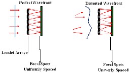
The main part of the AO system, as said above, is to detect the incoming distorted wavefront. For this an array of lenslet (Shack-Hartmann Lenslet Array) is used. The image, produced by the passage of light through this array onto a CCD, forms a spot pattern. Unlike an ideal plane wavefront which forms well focused equidistant spots, a distorted wavefront forms spots that are not equidistant as shown in Fig..2. Wavefront reconstruction is performed in two stages (1) slope calculation using image centroiding algorithms, (2) reconstruction of the wavefront shape from local slope measurement. Our first goal is to find the centroid of these spots based on an algorithm which is fast and accurate. From the centroid the wavefront is to be reconstructed through modal approach. Initially the system is focused on to a bright star or a laser guide, which acts as the reference. The reference image is taken and its centroid points are calculated. Next the system is focused on to the object of interest. After capturing the image of the object, the centroid is determined. There will be a shift in the centroid points when both the centroid points are compared of that of reference image and that of the image of the object.
Fig. 2: Lenslet Array with perfect and distorted wavefront
The shift may be in X direction or Y direction or in both the direction. From the knowledge of the focal length of the Shack- Hartmann lens and the distance of the centroid, the slope is determined. Deviation of spot position from a perfectly square grid measures shape of incoming wavefront. We used a very simple method to generate photon depleted spots. SHWS spot formed out of sufficient number of photons by a Gaussian shape. A two dimensional Gaussian function was simulated with control over the position at which the spot center lies. Sample ideal
spot images are shown in Fig. 3.The centroid of a sub aperture is calculated by the formula.
![]() (1)
(1)
Both Wx and Wy is a matrix whose size depends on the number of lenslets used to image the object of interest. Where f is focal length of the lenslet. and ∆x and ∆y are slope of the image in the x and y directions.
A. Algorithm for finding slope values and reconstruction of the wavefront.
1. Fixing of the origin for both the records (Reference and Aberrated images shown in fig.3)
2. Keeping the same origin determines the centroid of the spots in both the images.
3. Calculation of the slope of the wavefront at every co-ordinate
4. Fitting of the derivative of the Zernike polynomials
to the slope
5. Estimation of the Zernike coefficients by least
square fit
6. Wavefront reconstruction
7. Plotting of the wavefront surface (shown in fig.4)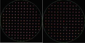
Fig.3 (a) reference spots (b) aberrated spots.
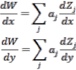
After finding out the centroid of each spot, the slope of the wavefront at each sub aperture is calculated with the knowledge of focal length of the Shack-Hartmann sensor and the deviation of the centroid of each spot from the reference image. From this slope the wavefront is reconstructed using modal approach. The aberrated wavefront has to be reconstructed from the wavefront slopes derived from the above method. The wavefront aberrations can be well represented by Zernike Polynomials. The derivatives of the Zernike polynomials can be expressed as a linear combination of Zernike polynomial [4]. The wavefront can be represented using Zernike Polynomial as:
![]() (2) Differentiating the above equation,
(2) Differentiating the above equation,
IJSER © 2013 http://www.ijser.org
International Journal of Scientific & Engineering Research, Volume 4, Issue 7, July-2013 98
ISSN 2229-5518
(3)
![]() (11)
(11)
![]() (12)
(12)
These can be rewritten as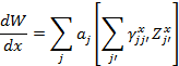
And hence it becomes,
(4)
(5)
(6)![]()
(13)
A provides the Zernike coefficients. Using the Zernike coefficients, the aberrated wavefront is reconstructed and plotted shown in Fig.4.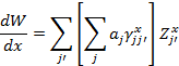
(7)
 (8)
(8)
The wavefront slope as derived from this method can be written as:
![]() (9)
(9)
![]()
Where ![]() correspond to the x and y derivatives of the wavefront slope. Now combining all these equations, we get:
correspond to the x and y derivatives of the wavefront slope. Now combining all these equations, we get:![]()
(10) In matrix notation this equation can be written as:
Where W contains the values of the wavefront slope, A the Zernike coefficients which are to be determined and Z is the Zernike polynomial corresponding to the coefficients. The number of measurements is typically more than the number of unknowns, so a least square solution is useful. This over determined system is solved as follows:
Fig. 4: The 2D representation of the wavefront error computed from the
Shack Hartmann method.
Shearing interferometry is another technique to measure wavefront phase through intensity measurements [5] for adaptive optics applications. Shearing interferometer using birefringent prisms have been described by Saxena and Lancelot [6, 7, 8] for wavefront sensing. This technique works on the basis of splitting a wavefront into two and recombining with one wavefront slightly displaced. The basic approach is to produce an interference pattern between the wavefront and a sheared or displaced replica of itself. Polarized Shearing Interferometer (PSI) uses a single interferogram to determine the wavefront error. The resulting interference patterns record wavefront tilt and allow wavefront reconstruction from partially extended sources. In this, the phase variations, which cannot be measured directly because of its high temporal frequency, are converted into intensity variations (fringe pattern) in the pupil plane. Like Shack Hartmann sensor, Shearing interferometry measures the wavefront slope. Shearing interferometry has the important advantage that it requires no reference wavefront for the production of fringes other than the incident wavefront itself. It is important to understand the Polarization Shearing Interferometer (PSI) theoretically to sense the wavefront errors. For this purpose a simulation of wavefront has been generated using Zernike polynomials and incorporated the wavefront errors caused due to atmospheric turbulence with varying noise levels and atmospheric turbulence. The theoretical
IJSER © 2013 http://www.ijser.org
International Journal of Scientific & Engineering Research, Volume 4, Issue 7, July-2013 99
ISSN 2229-5518
simulation helps one to understand the behaviour of the fringe patterns in different circumstances.
In a telescope imaging system, the major sources of error, is from the atmospheric turbulence apart from other sources like, fabrication error and noise. A wavefront sensor computes these wavefront errors in real time and sends the signals for the control computer for adaptive correction. It is important to understand the Polarization Shearing Interferometer theoretically and its efficacy to sense the wavefront errors and its limitations. A systematic theoretical study has been undertaken. The wavefront was generated using Zernike polynomials and the wavefront errors caused due to atmospheric turbulence was incorporated. From these simulation studies the optimum parameters for which the PSI wavefront sensor could be used in AO system has been derived. Simulations were also carried out with varying noise levels and atmospheric turbulence. Simulations were carried using LABVIEW.
Zernike polynomials are widely used for describing the classical aberrations of an optical system [9]. They have the advantage that the low order polynomials are related to the classical aberrations like, spherical aberration, coma and astigmatism. Fried [10] used these Zernike polynomials to describe the statistical strength of aberrations produced by the atmospheric turbulence. Zernike polynomials are a set of orthonormal polynomials, defined on a unit circle and hence are convenient to express the turbulent wavefront in the circular aperture telescope. Noll [4] has introduced a normalization for the Zernike polynomials that is perfectly suited for application of Kolmogorov turbulence. The use of Zernike polynomials for describing the wavefront aberrations introduced by the atmospheric turbulence is a well established fact. Since this wavefront sensor measures the wavefront slope, it is imperative to represent the Zernike polynomials in its derivative form. The derivatives of the Zernike Polynomials as a linear combination of Zernike polynomial is given by Noll [4] which are reproduced below. The gradient of the Zernike polynomial is represented and the wavefront slope is explicitly written as
[4], representing different aberrations in units of wavelengths.
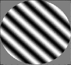
the ideal conditions are described as the system having no aberrations and system with aberrations are shown in Fig.5.a and Fig.5 b.
(a)
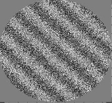
(b)
Fig.5 (a) A Noise-free fringe pattern (b) A noisy fringe pattern
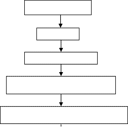
The data analysis of the PSI interferometric data has been carried out in the Lab View platform. The following methodology as shown in Fig. 6 has been adopted.
Image Rotation
n
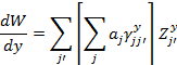
∆W ( x, y) = ∑ a j s∑γ x jj' Z j' + t ∑γ y jj' Z j'
j =1
j'
j'
(14) Where
2D FFT
γ jj′ is called Zernike Derivative matrix. Using the above
expression and assuming equal shear values for both the X
and Y directions interferograms are simulated for different values of the Zernike coefficients, whose values are given in (NOLL) In the case of Polarization Shearing Interferogram,
IJSER © 2013 http://www.ijser.org
Noise Elimination
Identification of carrier Frequency
Shift of carrier frequency side to the origin
International Journal of Scientific & Engineering Research, Volume 4, Issue 7, July-2013 100
ISSN 2229-5518
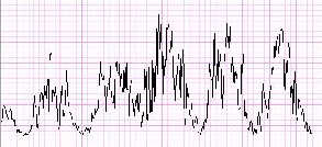
Fig.7.a A typical one dimensional noisy interferogram profile
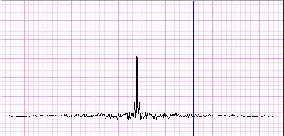
Fig.7.b Fourier Transform of the interferogram
Fig.6 Flow chart of the methodology adopted
A. Wavefront error estimation from a Single Fringe Record
This part is devoted to the analysis of a single PSI
interferogram to estimate errors for appropriate correction for an AO system. Fourier analysis approach has been adopted for determination of local phase of the proposed PSI interferogram. The Fourier transform method is resistant to noise and is highly efficient and very simple to apply. The phase thus recovered is measured with an integral multiple of 2π uncertainties. The process of removing these uncertainties is called phase unwrapping.
Wavefront determination from wavefront slope data using
Zernike polynomial
After phase has been completely unwrapped, the data contains the derivatives of the original phase of the wavefront. The derivative of the wavefront phase can conveniently be written in terms of Zernike polynomials, to estimate the wavefront errors. The Zernike coefficients provide the complete information of the wavefront. The aberrated wavefront has to be reconstructed from the wavefront slopes derived from the above method. The wavefront aberrations can be well represented by Zernike polynomials. The derivatives of the Zernike polynomials can be expressed as a linear combination of Zernike polynomial (Noll, 1976). They are written as
∆Z j = ∑γ jj' Z j'
Fourier transform methods offer greater flexibility in the
separation of the low frequency and high frequency
components in the spatial frequency spectrum. The
irradiance distribution in an interferogram can be described
j'
Alternatively
∆j =
a γ Z
(16)
∑ ∑
j jj' j'
as j' j
(17)
I (x, y) = A(x, y) + B(x, y) cos [2π fo .r + f (x, y)] (15)
where A(x,y), and B(x,y), are the unwanted irradiance
variations arising due to the imperfections in the optical
system, and Ø(x,y) represents the phase of the
When the shear value in X and Y directions are small, the resultant sheared wavefront can be approximated as the first order derivative function as
∆W ( x, y) = ∂w s + ∂w t
interferogram and
fo is the spatial carrier frequency. A
![]()
![]()
∂x ∂y
(18)
typical one dimensional irradiance distribution of an
interferogram and its Fourier transform is shown in Fig. 7.a
and 7.b.
∂W
![]()
where ∂x
∂W
![]()
& ∂y
correspond to the x and y derivatives
of the wavefront slope. Therefore
IJSER © 2013 http://www.ijser.org
International Journal of Scientific & Engineering Research, Volume 4, Issue 7, July-2013 101
ISSN 2229-5518
![]()
∂W =
∑ ∑
a jγ jj'
Z j'
The software for the analysis of the Polarized Shearing
∂x
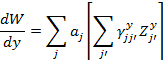
![]()
∂W =
j' j
a γ
and (19)
y
Z
Interferogram and Shack Hartmann images was written in the LabView platform. An in-depth, study has been made for the application of PSI method for AO. Fourier
∑ ∑
j jj' j'
∂y j' j
(20)
theoretical approach has been applied to this configuration
So that combining (18), (19) and (20),
to establish the basis of the wavefront sensing. Theoretical
simulations were carried out for visualization of various
∆W (x, y) = s∑ ∑ a jγ jj'
j' j
Z j' + t∑ ∑ a jγ jj'
j' j
y
Z j'
(21)
aberrations in the interferometric fringe pattern. The study reveals that under moderate turbulent conditions the sensitivity of PSI is reasonably good for adaptive optics
In matrix notation this equation can be written as
W = A Z
Where W contains the values of the wavefront slope, A the Zernike coefficients which are to be determined and Z is the Zernike polynomial corresponding to the coefficients with a multiplicative factor of shear. After removing the x-tilt and y-tilt and the defocus term the wavefront is recomputed using the Zernike polynomials. Using least square solution this over determined system was solved. The 2 dimensional wavefront error computed is shown in Figure 8. The Zernike coefficients are compared for both SH-WS and PSI- WS (Fig.9) in the bar diagram.
applications. Since this operates in the intensity mode, high
spatial sampling is possible. The speed is governed by the
computation time, which can be largely improved. The
convenience of the size, the ease of operation and
insensitivity to vibrations, makes this device as a suitable
wavefront sensor for adaptive optics application. Hence we conclude that the lateral shearing interferometer is cost effective and very easy to integrate into an adaptive optical system for wavefront sensing with large spatial distribution limiting only to detector’s characteristics.
1. [1] J. W. Hardy, Adaptive Optics for Astronomical Telescopes, Oxford
University Press, New York, (1998).

2.
3. [2] Roddier F. Curvature sensing and compensation: a new concept in adaptive optics, Appl.Opt., Vol. 27, No.7, 1223 – 1225, (1988).
4.
5. [3] Ben C Platt and Roland Shack, History and Principles of Shack- Hartmann Wavefront Sensing, Journ. of Refr. Surg. Vol. 17, S573 – S576
(2001).
6.
7. [4] Noll, R.J., Zernike polynomials and atmospheric turbulence, J. Opt.
Soc. Am., Vol. 66, No.3, 207 – 211 (1976).
8.
9. [5] Jeffrey D Barchers, David L Fried, and Donald J Link, “Evaluation of the performance of a shearing interferometer in strong scintillation in the absence of additive measurement noise”, Appl. Opt. Vol. 41, No.18, 3674
– 3684 (2002)
Fig. 8. The 2D representation of the wavefront error computed from the
Shack Hartmann method.
10.
11. [6] Sandler, D G., Cuellar, M Lefebvre. T Barrett, R. Arnold, P. Johnson, A.
Rego, G. Smith, Z.Taylor and B.Spivey., Shearing interferometry for laser- guide star atmospheric correction at large D/ro, J. Opt. Soc. Am. A., Vol.11, No.2, 858 – 873 (1994).
12.
13. [7] Saxena A.K, Quantitative Test for concave aspheric surfaces using a
Babinet Compensator, Appl. Opt. Vol. 18, No.16, 2897 – 2901, (1979).
14.
15. [8] Saxena A.K, and Lancelot J.P, Theoretical fringe profiles with crossed Babinet compensators in testing concave aspheric surfaces, Appl. Opt. Vol. 21, No.22, 4030 – 4032 (1982).
Fig.9. A comparitive plot of the 20 Zernike coefficients computed by the
SH and PSI method.
16.
17. [9] Born E and Wolf, “Principles of Optics” Pergamon Press. (1970).
18.
19. [10] Fried, D.L. “Statistics of a geometrical representation of wavefront
IJSER © 2013 http://www.ijser.org
International Journal of Scientific & Engineering Research, Vo lume 4, Issue 7, July-2013
ISSN 2229-5518
distortion"J.Op!Soc.Am, Vol55, No.ll,1427-1435 (1965).
102
1-BER IS)2013