have performed classification.
International Journal of Scientific & Engineering Research, Volume 4, Issue 6, June-2013 522
ISSN 2229-5518
Performance Comparison of Classification Algorithms employed in Data Mining
Jyoti Chauhan, Dr Udayan Ghose
Abstract— Extracting information from past data and using it to predict future events by capturing relationships between explanatory and predicted variables is called Predictive Analytics. Various data mining techniques (like Classification, Association, Feature Extraction, Clustering, etc.) and related algorithms employed in predicting future events help us to solve various business and day-to-day problems. In this paper we shall focus on Predictive Analysis Operations and algorithms involved in the technique of Classification and evaluate the performance of each in solving the “Targeting the Right Customer” problem faced by Insurance industries, using a sample Insurance Customer database. We shall apply all the classification algorithms (Naïve Bayes, Decision Trees, Support Vector Machines, Generalized Linear Model) on this sample Insurance DB and compare the results obtained from each to finally determine the algorithm that best solves the problem of identification of right customer. The work would involve stages like exploring the customer database, performing Classification of existing customers into 2 groups – those who would buy the new insurance policy and those who would not buy, by applying different algorithms and then finally determining the best algorithm based on parameters like predictive confidence, average and overall accuracy ,etc.
Index Terms— Classification, Data Mining, Decision Trees, Generalized Linear Model, Insurance, Naïve Bayes, Predictive Analytics, Support Vector Machines, Targeting Right Customer
—————————— ——————————
Accurate forecasting of factors like budget, product inven- tory and demand, supplies, and operations play a vital
role in determining any organization’s success. All these in turn depend on the application of various predictive tech- niques and model that analysts in an organization deploy on the existing data to churn predictions of future events. The more accurate the applied tools and mechanisms are, the higher is the reliability of the results obtained.
Predictive Analytics is a branch of statistical analysis used for forecasting and modeling. It deals with extracting infor- mation from past data by capturing relationships between explanatory and predicted variables, and then using it to pre- dict future behavioral patterns and trends [1]. We shall take a small overview of the use of Predictive Analysis in a variety of industries.
a. Marketing Industry: Proper data mining algorithms and predictive modeling not only narrow a users tar- get audience but also allows users to tailor their ads with respect to each online customer as per the way the customer navigates their site [1]. The marketing team thus gets the opportunity to develop multiple advertisements based on the past clicks of their visi- tors. Predictive analytics can aid in choosing market- ing methods, and marketing more efficiently [2].
————————————————
b. Insurance Industry: Predictive operations gain much more importance especially when the industry is the one which deals with handling and movement of money at all points of time like an Insurance Industry. Insurance industry has always relied on forecasting [1]. Forecasting premiums and targeting best custom- er - what initially started as a simple guessing phe- nomenon with the advent of technology and in an ex- tensive search for accurate results ultimately emerged as the best insurance industry practice of employing predictive analytics.
c. Data warehousing Industry: As per Hugh and Barba- ra [3] stated in their work, “Getting data in is the most challenging aspect of BI, requiring about 80 percent of the time and effort and generating more than 50 per- cent of the unexpected project costs.” Oracle Data Mining also offers Data Cleansing functions which help remove redundant and erroneous data from the data sources before being used for any other purpose.
d. Population Analysis: Analysts keep studying the
population and events in a given geographical area
and the emerging trends and pattern of the popula-
tion in the region. As per the statement by Ross, Ryan and Stephen [4] in their work “As event data are cap- tured, algorithms and analysts search for unexpected events, and these unexpected events then trigger an alert. Application of predictive analytics to such data helps generate a kind of syndromic surveillance which tries to convert a reactive paradigm to a proac- tive paradigm [4].
e. Social Media Analytics: Roosevelt C. Mosley [5] in his paper on analyzing the Insurance Twitter posts has emphasized on the various concepts of data mining
IJSER © 2013 http://www.ijser.org
International Journal of Scientific & Engineering Research, Volume 4, Issue 6, June-2013 523
ISSN 2229-5518
like data cleansing, clustering, and classification ap- plied to Twitter posts. Data mining functionalities on social media can help related industries to proactively address potential market and customer issues more effectively [5].
f. Medical Industry: The type of data and the question raised may vary from one industry to other. Depend- ing on the data and the problem statement to solve, the data analysis might include the application of sta- tistical methods or other techniques [6]. Certain sub- sets of data may be selected or discarded depending on requirements. Cheu Eng Yeow [6] in his work has employed the Naïve Bayes Classifier to classify the Liver Disorders dataset and the importance of various attributes in alcohol induced liver disease. Similarly predictive analysis can be applied to Stock exchanges to predict better return yielding stocks for future.
All the present day industries have huge amount of histori- cal data along with case studies which carry a lot of infor- mation. The general idea that “Data is critical and can be put to future use” is familiar with all the data divisions of these industries but how it can be achieved is still a big matter of concern. The problem is that not all of these industries are able to process and analyze this precious information from the past for predicting a better future. Some of them keep piling loads of data for long years until a time comes when they finally decide to discard this data by declaring it to be “of no-use”.
Industries like insurance, medical and credit industries are the ones who suffer major losses because of lack of ways and instruments to analyze their past data. Manual analysis of data in databases or files on a large scale doesn’t produce much fruitful results and is also a time consuming activity. This cre- ates a need for data mining algorithms and some form of pre- dictive modeling which could be applied to this historical data in databases for guiding future actions.
In the absence of proper data mining algorithms and predic- tive models following events occur very often:-
• Proper identification of a target audience/ customer for a product becomes difficult.
• The amount of money spent in closing a sale deal is high.
• Not much or little attention is being paid to customer demographics (i.e. customers for an organization are growing older or younger [4]).
• Marketing team is not able to narrow down what ad- vertisement to be directed to which customer.
In Credit industries, the Credit rating of a loan seeking in- dividual can be determined based on his past data records. In Insurance industries, proper data mining helps the Insurance agents to divert their energy and resources to those individu- als who are more likely to buy insurance. In Medical indus- tries, the effectiveness of a given medicine in curing a particu- lar disease, the results of following a particular treatment or- der for curing a sickness and other such related data produce high quality measures which could be promoted and followed in future for effective treatments and results.
Classification is the most commonly used technique for predicting a specific outcome based on historical data. The various classifications for an Insurance industry customer, which can form different problem statements for an analyst, are of the form as listed underneath:
1. response / no-response
2. high / medium / low-value customer
3. likely to buy / not buy
As part of this dissertation work on ‘Performance Compari- son of Classification Algorithms employed in Oracle Data Mining’, we will solve the ‘Targeting the Right Customer’ problem faced by Insurance industries. For this work we shall take a sample ‘Insurance Customer’ database (DB) in Oracle, on which we would apply the Classification function from the class of available Oracle Data Mining functions in SQL Devel- oper 3.0.
The Classification function in SQL Developer 3.0 can be implemented using any of the below listed 4 algorithms:
• Generalized Linear Model (Binary Logistic
Regression)
• Naïve Bayes
• Support Vector Machine
• Decision Tree
We shall understand the theory for each of the four algo- rithms and their way of working. Next we shall explore the sample Insurance Customer DB to determine whether any useful interpretation can be made out of it using the SQL De- veloper’s ‘Explore Data’ function. Later on we will apply all the classification algorithms on this sample Insurance DB and compare the results of each algorithm on the basis of the be- low listed parameters:
• Performance Measures
Predictive Confidence (%)
Average Accuracy (%)
Overall Accuracy (%)
• Performance Matrix (Confusion Matrix or Actual vs.
Predicted Matrix)
• Receiver Operating Characteristics (ROC), a plot of
False Positive Fraction vs. True Positive Fraction
• Lift (degree to which the predictions of a classification model are better than randomly-generated predic- tions)
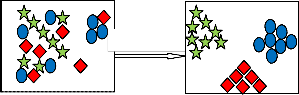
Classification as the word suggests is the basic process of iden- tifying and grouping objects with the same functionality and features into a single group called as a class. It can also be re- lated to the concepts of Object Oriented Programming where objects of a class have similar attributes and functionalities with their individual data value being different. Taking a gen- eral example we can say that if we have a bundle of books belonging to different subjects say English, Hindi, Mathemat- ics, and Science lying on a table, then if we are able to sort and create separate groups of books belonging to each subjects we
IJSER © 2013 http://www.ijser.org
International Journal of Scientific & Engineering Research, Volume 4, Issue 6, June-2013 524
ISSN 2229-5518
have performed classification.
Classifica-
Fig.1. Classification
If we talk of the similar concept in terms of data in a data- base, we would describe Classification process as given below by Tan, Steinbach and Kumar [8]:
Given a collection of records (training set)
– Each record contains a set of attributes; one of the
attributes is the class [8].
By the above statement we mean that for the given data set, the class assignments are available as one of the attribute. We need to find a model for this class attribute such that the class attribute can be expresses as a function of the values of other attributes [8]. The model so obtained should then be used to assign any new set of record to one of the identified set of clas- ses with a high level of accuracy. The Accuracy of the model is determined by using a Test Set. In Oracle Data Mining, the data set under consideration is divided into two sets, namely Training and Test. The model is created using the training set and validated using the test set.
The attributes or features of a class can be divided into the following types:
(1) Quantitative features [12]:
(a) Continuous values (e.g., height, weight [12]);
(b) Discrete values (e.g., the number of computers, keyboards, mouse [12]);
(c) Interval values (e.g., the duration of an event). (2) Qualitative features [12]:
(a) Nominal or unordered (e.g., color);
(b) Ordinal (e.g., military rank or qualitative evalua-
tions of temperature (“cool” or “hot”) or sound inten-
sity (“quiet” or “loud”)).
Classifications result in discrete values and it does not im- ply ordering of any sort. Depending on the kind of target at- tribute or problem the predictive model is chosen. Like for a numerical target the predictive model would uses a regression algorithm, instead of a classification algorithm. In general, there can be 2 types of classifications – Binary classification and Multiclass classification. Only two values are possible for the target attribute in case of binary classification: say, customer buys insurance or does not buy insurance. More than two tar- get class values exist in case of multiclass classification: for example, customer may belong to any of the credit rating clas- ses like low, medium, high, or unknown.
A classification algorithm detects the relationships that ex-
ist between the predictors and the target attributes during the model build (training) phase. The techniques for finding rela- tionships differ for different classification algorithms. The rela- tionships between attributes for a given class are summarized in a model, which are later applied to fresh or new data sets in which the class assignments are unknown to detect their clas- ses.
The models created during the training phase are tested by comparing the predicted values to known target values in a set of test data. In the Scoring process of a classification model, class assignments and probabilities for each record in the test data would also be determined. For example, an insurance classification model that would classify customers on credit rating parameter as low, medium, or high value would also predict the probability of each classification for each customer. The accuracy of a model in predicting the outcomes is meas- ured based on certain values which are known as Test metrics.
Accuracy
Accuracy refers to the percentage of correct predictions made by the model when compared with the actual classifications in the test data [11].
Confusion Matrix
A confusion matrix displays the number of correct and incor- rect predictions made by the model compared with the actual classifications in the test data [11]. For a binary classification model the confusion matrix is a 2-by-2 matrix. In case of classi- fication resulting in multiple classes (say, n) the resultant ma- trix is a square matrix of size n-by-n. The rows of the matrix denote the count of actual classifications in the test data whereas the columns denote the count of predicted classifica- tions which are made by the classification model under con- sideration. Fig. 2 below shows the Confusion Matrix for a bi- nary classification model. The results ‘Yes’ can also be identi- fied by number 1 and the results ‘No’ can be identified using number 0.
Fig.2. Confusion Matrix for a Binary Classification Model
The following information can be derived from a confusion matrix:
• Correct predictions (a+d).
IJSER © 2013 http://www.ijser.org
International Journal of Scientific & Engineering Research, Volume 4, Issue 6, June-2013 525
ISSN 2229-5518
Lift
• Incorrect predictions (b+c).
• Total scored cases (a+b+c+d).
• Error rate (b+c)/(a+b+c+d)
• Overall accuracy rate (a+d)/(a+b+c+d)
verse proportion to the changes in probability threshold. For example, if the threshold for predicting the positive class is raised from a value of 0.6 to 0.7 then it will result in fewer pos- itive predictions. It will also affect the numbers of true/false positives and true/false negatives to change for the given model.
ROC can be used to find the probability thresholds that
This metric is a measure of winning edge that predictions
from a classification model can provide over any randomly-
generated predictions. Lift can only be calculated in case of
binary classification. In case a model has multiple classes, then
we can convert it to a binary model by identifying one of the
available class as a positive class and the other classes as nega-
tive results from the model.
In mathematical terms, Lift can be defined as a ratio of two percentages: the percentage of correct positive classifications made by the model to the percentage of actual positive classi- fications in the test data [11].
Receiver Operating Characteristic (ROC)
All classification models use a decision point known as proba- bility threshold for the purpose of making decisions, default value being 0.5 for binary classification. ROC measures the impact of changes in the probability threshold [11]. It is very similar to Lift and applies only to binary classification models. ROC provides the user with an insight about the chances with which the model would accurately predict the negative or the positive class for a given data or record.
The ROC Curve
ROC Curve is defined as the ratio of false positive rate (placed on X-axis) to the true positive rate (placed on the Y-axis) where true/false positive rate/fraction is described as below:
True positive fraction [11]: Hit rate. (True positives/ (true posi- tives + false negatives))
False positive fraction [11]: False alarm rate. (False positives/ (false positives + true negatives))
Area under the Curve
It refers to the area under the ROC curve (AUC) which measures the likelihood of a binary classification model in identifying a given actual positive case of being positive, ra- ther than an actual negative case, with higher probability. For data sets suffering from unbalanced target distribution this measure is highly useful.
ROC and Model Bias
The predictions made by a classification model change in in-
yield the highest overall accuracy or the highest per-class ac- curacy [11]. A Cost matrix is a convenient mechanism for changing the probability thresholds for model scoring.
Following are the major Data Mining Classification algorithms under consideration for solving the “Targeting the Best Cus- tomer Problem” under consideration:
• Decision Tree - Decision trees automatically generate rules, which are conditional statements that reveal the logic used to build the tree [11].
• Naive Bayes - Naive Bayes uses Bayes' Theorem, a formula that calculates a probability by counting the frequency of values and combinations of values in the historical data [11].
• Generalized Linear Models (GLM) - GLM is a popular statistical technique for linear modeling. Oracle Data Mining implements GLM for binary classification and for regression [11]. GLM provides extensive coeffi- cient statistics and model statistics, as well as row di- agnostics. GLM also supports confidence bounds [11].
• Support Vector Machine - Support Vector Machine (SVM) is a powerful, state-of-the-art algorithm based on linear and nonlinear regression. Oracle Data Min- ing implements SVM for binary and multiclass classi- fication [11].
The nature of the data determines which classification algo- rithm will provide the best solution to a given problem. The algorithm can differ with respect to accuracy, time to comple- tion, and transparency. Practically we can develop several models for each algorithm, select the best model for each algo- rithm, and then choose the best of those for deployment.
A decision tree is a powerful and popular tool that uses a tree- like graph for decision making process. Decision trees are used to predict possible consequences of certain actions. It is most commonly utilized in the field of operations research to identify goal-oriented strategies, event outcomes, resource utility and costs. It is one way to display an algorithm which is
IJSER © 2013 http://www.ijser.org
International Journal of Scientific & Engineering Research, Volume 4, Issue 6, June-2013 526
ISSN 2229-5518
based on conditional probabilities. Decision trees generate rules which are conditional statements in human readable and understandable form, which can be used to identify a set of records within a database. Rules not only provide an inside view of the working predictive model but also introduce transparency in the decision making process. In other words, they form the building blocks for the predictive model.
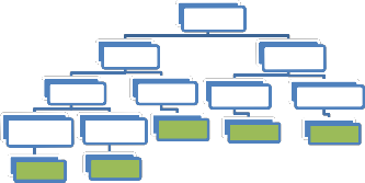
Target values in a decision tree are predicted through a se- ries of questions which follow a particular sequence. The im- portance of sequence simply dictates that the questions asked at any given stage directly depend upon the answers to the questions asked in the previous stage. The main aim is to ask questions such that it leads to the identification of unique and specific target values, forming a graphical tree like structure. The fig. 3 displays a sample binary classification tree for solv- ing the ‘Targeting the Right Customer’ problem for the insur- ance industry. Here we have 3 attributes under consideration
– Insured {Yes, No}, Married {Yes, No}, Has Children {Yes, No}
and we make predictions for the attribute Buy Insurance {Yes,
No}. The text in red color in all the boxes denotes the answers
to questions at the previous level. The text boxes in green color
denote the final classification results reached. The set of deci-
sion rules that represent the decision tree in example are:
• IF (INSURED = “YES” AND MARRIED = “YES” AND HAS_CHILDREN = “YES”) THEN BUY_INSURANCE = “YES”
• IF (INSURED = “YES” AND MARRIED = “YES” AND HAS_CHILDREN = “NO”) THEN BUY_INSURANCE = “NO”
• IF (INSURED = “YES” AND MARRIED = “NO”) THEN BUY_INSURANCE = “NO”
• IF (INSURED = “NO” AND MARRIED = “YES”) THEN BUY_INSURANCE = “YES”
• IF (INSURED = “NO” AND MARRIED = “NO”) THEN BUY_INSURANCE = “NO
multiple classes i.e. it can be sued to solve both binary and multiclass classification problems. The test conditions (or Rules) can be specified based on the following two factors:
• Depending on the types of Attributes
• Depending on the type of Classification to be per- formed
3.1.1 Attribute types
The kinds of attributes that describe a given entity also play a key role in determining the classification results. We have the below types of attributes:
* Nominal (categorical attributes with no fixed order, Exam- ple: viral infections could be {cough, sore throat, cold} [13])
* Ordinal (categorical attributes with fixed order, Example: Temperature can be classified as {Extreme Cold, Cold, Moder- ate, Hot, Extremely Hot} with the rising order of temperature being Extreme Cold < Cold < Moderate < Hot < Extremely Hot)
* Continuous (numerical values like height, weight, salary etc form a part of these attributes)
3.1.2 Classification types
A decision tree can be used to perform the below two types of classifications:
* Binary Classification - It aims at performing a two-way split of the classification attribute under consideration. In case, the attribute has multiple classifications possible grouping of the attribute is done to form 2 classes as per the requirement. The figure shown above is an example of binary classification.
* Multiple Classifications - In this the attribute under consid- eration is split into multiple classes as shown in the fig. 4 be- low:

Insured ?
"Yes" Has
children?
"Yes" Married ?"No"
Buy
Insurance
"Yes" Buy
Insurance
?
"No" Married?
"No" Buy
Insurance?
"Yes"
Buy
Insurance?
YES
"No" ?
Buy NO Insurance?
NO
YES NO
Hot (> 37°C)
Moderate (25°C Cold (< 25°C)
to 37°C)
Fig.3. Sample Decision Tree (Binary classification) for ‘Target- ing the Right Customer’
The Decision Tree algorithm produces accurate and inter- pretable models with relatively little user intervention [11]. This algorithm can be used to split data into both binary and
Fig.4. Multiple Classifications
One of the most important steps in the classification pro- cess using a decision tree is to perform the splitting of the rec- ords into two child nodes repeatedly in an efficient manner. For calculating the splits, Oracle Data Mining offers two ho- mogeneity metrics - gini and entropy, [10] default being gini.
IJSER © 2013 http://www.ijser.org
International Journal of Scientific & Engineering Research, Volume 4, Issue 6, June-2013 527
ISSN 2229-5518
Homogeneity metrics, also referred to as Purity, perform the task of assessing the quality of alternative split conditions and promoting the selection of that split which would result in the formation of the most homogeneous child nodes. It is a measure of the degree to which records with same target value form a part of the resulting child nodes. It aims at maximizing the purity of the child nodes. For example, if the target classi- fication result can be a binary value of the form yes or no, the objective of the gini would be to produce nodes where majori- ty of the cases will be either Yes or No. The below formula is used for calculating Gini Index for a given node‘t’ [8]
𝐺𝐺𝐺𝐺(𝑡) = 1 − ∑𝑗[𝑝(𝑗|𝑡)]2 (1)
Where, p (j | t) is the relative frequency of class j at node t
[8].
Example, Consider the below binary classifications
For Example 1a, GINI = 1 – [(0/7)2 + (7/7)2] = 0.00 (Infor- mation of High Interest)
For Example 1b, GINI = 1 – [(1/7)2 + (6/7)2] = 0.24
For Example 1c, GINI = 1 – [(3/7)2 + (4/7)2] = 0.5 (Infor- mation of Least Interest)
belong to one class then the node has the maximum infor- mation. In other words, both Entropy and GINI are very simi- lar computations.
Different applications of data mining aim at providing dif- ferent level of solutions. While some of the applications are prediction-accuracy oriented irrespective of the working model. Others, may be decision-reason oriented banking on the reasons based on which a decision was made and may require exten- sive explanation. For example, to ensure the complete success of a marketing campaign for a new insurance policy to be launched, the Marketing professional would not only be re- quired to present his choice of customer segment for the new policy but would also need in-depth knowledge and descrip- tions of the available customer segments in the current data- base. For such a scenario, the Decision Tree algorithm for pre- dictive analytics would be an ideal choice.
In a practical scenario, any Decision Tree algorithm grows each branch of the tree only till the extent that it is able to per- fectly classify the training examples [11]. In some situations like noisy data or too small a training set, it may lead to an Over-fitting problem wherein the predictive classification model is able to predict accurately only the training data and any new data presented remains unclassified. Care should be taken to avoid such a situation.
The Naive Bayes algorithm has its roots deep inside the Bayes Theorem which states that given the probability of a prior event, the probability of occurrence of another event depend- ent on the prior event can be found. In other words we can say that Naïve Bayes algorithm is based on conditional probabili- ties [11]. As per Bayes' Theorem, probability is calculated by counting the frequency and combinations of values in the data set under consideration. In a statement form, if D represents a dependent event and P represents the prior event, then as per Bayes' theorem we have:
Higher the value of GINI, higher is the impurity of a node
𝑃𝐸𝐸𝑃(𝐷 𝑔𝑔𝑔𝑔𝐸 𝑃) = 𝑃𝐸𝐸𝑃(𝑃 𝑎𝐸𝑎 𝐷)⁄𝑃𝐸𝐸𝑃(𝑃)
(3)
and less recommended is the split resulting in this value. A lower value of GINI indicates higher purity of the node and better split decision.
Entropy is a measure of the information content of the source and is also used for measuring the homogeneity of a node. As per Tan, Steinbach and Kumar, Entropy at a given node t is given by the below formula:
To find the probability of dependent event D occurring giv-
en prior event P has already occurred, we divide the count of
the number of cases where P and D occur together by the
number of cases where P occurs alone.
Suppose our task is to predict the chances that a customer under age of 21 will buy an insurance policy. For this scenario,
‘under age of 21’ will form the prior condition (P) and ‘buy in- surance’ will be the dependent condition (D). We shall materi-
𝐸𝐸𝑡𝐸𝐸𝑝𝐸 = − ∑𝑗 p(j|t) log2 p(j|t)
(2)
alize this example by assuming a total of 500 customers in the training data set with 125 of them being less than 21years of
Where, p (j | t) is the relative frequency of class j at node t
[8].
A given node contains least information if the records are
equally distributed among all classes whereas if all records
age and 100 of them interested in buying an insurance policy. For this case, we have:
Prob (P and D) = 100/500 = 20%
IJSER © 2013 http://www.ijser.org
International Journal of Scientific & Engineering Research, Volume 4, Issue 6, June-2013 528
ISSN 2229-5518
Prob (P) = 125/500 = 25%
In this Bayes' Theorem would lead to the prediction that
80% of customers under the age of 21years are likely to buy an
insurance policy (20/25). Certain special terminologies associ-
ated with the Bayes Theorem are:
• Pairwise – Cases where both prior P and depend- ent D conditions occur together
• Singleton – Cases where only the prior condition
P occurs
With respect to the above terms, a Naive Bayes algorithm determines the probability as a result of the division of the % of pairwise occurrences by the % of singleton occurrences [11]. Very small values of predictor or prior percentages do not contribute to the model effectiveness. Usually a threshold val- ue is set to ignore such very small values during the calcula- tion process.
The above example is a very simple one which depicts a dependent event D based on a single independent event P. However, in case of Naïve Bayes algorithm the dependent event D is based on multiple independent events say {P1,P2,
…,Pn} i.e. each predictor or prior event is conditionally inde- pendent of the other predictors [11]. The general statement for
Naïve Bayes algorithm can be expressed as:
𝑃𝐸𝐸𝑃(𝐷|𝑃1, 𝑃2, … , 𝑃𝐸) =
West} could be used).
The Naive Bayes algorithm offers the following advantages:
1. Speed (It is fast.)
2. Highly scalable model building and scoring [11].
3. Linear scaling with the number of predictors and
rows [11].
4. Parallelized build process
5. Useful for both binary and multiclass classification
problems [11].
Generalized Linear Model (GLM) is a model which is used to express a dependent variable D as a linear combination of a given set of explanatory or predictor variables P {x1, x2, …,xn} as per the below equation:
f(D) = β0 + β1x1 + β2x2 + … + βpxp (9)
For some datasets, where the dependent variable (D) is con- tinuous and can be assumed to be having a reasonably normal distribution, it isn’t transformed at all and a multiple linear regression analysis can be performed. However, for datasets where the dependent variable D is binary (i.e. 0/1) like buys insurance – 1 and doesn’t buy insurance – 0 logistic regression is performed, using the logit or logistic function. Oracle Data Mining Operations uses Binary Logistic Regression for per-
𝑃𝐸𝐸𝑃(𝐷)𝑃𝐸𝐸𝑃(𝑃1, 𝑃2, … , 𝑃𝐸|𝐷)⁄𝑃𝐸𝐸𝑃(𝑃1, 𝑃2, … , 𝑃𝐸)
We derive the above equation from the below equation:
𝑃𝐸𝐸𝑃 (𝐴|𝐵) = 𝑃𝐸𝐸𝑃 (𝐴 𝑎𝐸𝑎 𝐵)⁄𝑃𝐸𝐸𝑃 (𝐵)
𝑃𝐸𝐸𝑃 (𝐵|𝐴) = 𝑃𝐸𝐸𝑃 (𝐵 𝑎𝐸𝑎 𝐴)⁄𝑃𝐸𝐸𝑃(𝐴)
(4)
(5) (6)
forming classification operation.
When the response variable has several categories a model that allows for several categories in the response variable such as multinomial regression [14] can be used. Alternatively the response variable can be recoded to produce two categories and perform a binary logistic regression analysis. However, statistically it will not be as efficient as performing a true mul- tinomial analysis.
𝑃𝐸𝐸𝑃 (𝐴 𝑎𝐸𝑎 𝐵) = 𝑃𝐸𝐸𝑃 (𝐵 𝑎𝐸𝑎 𝐴) (7)
From Equations, (5), (6) and (7) we get Equation (8) as:
Before getting into the details for Binary Logistic Regres- sion algorithm we must understand the some basic concepts related to proportions, probabilities and binomial distribution.
𝑃𝐸𝐸𝑃(𝐴|𝐵) = 𝑃𝐸𝐸𝑃(𝐴)𝑃𝐸𝐸𝑃(𝐵|𝐴)⁄𝑃𝐸𝐸𝑃(𝐵)
(8)
Proportions and probabilities differ from continuous variables [14] in a lot many ways. Both proportions and probabilities are bounded by 0 and 1in contrast to continuous variables whose
Even if the independence assumption is violated in a prac-
tical scenario, the model’s predictive accuracy isn’t significant-
ly degraded and makes Naïve Bayes a fast, computationally
feasible algorithm [11].
Data input for a Naive Bayes classification algorithm usual- ly requires binning which reduces the cardinality of various data columns to appropriate values. Say, for example continu- ous values like salary could be binned into ranges of the form
– {high, medium and low} whereas categorical data could be binned into classes which are one level higher than current (for example, instead of cities regions like {North, South, East,
values can be anything between plus or minus infinity. This simply emphasizes that proportions have no normality but a binomial distribution.
In cases of a normal distribution, the mean and variance are independent values. But in case of Binomial distribution the mean and variance are not independent of each other.
• For a Binomial Distribution, the mean is denoted by P and the variance by P*(1-P)/n, where n is the number of observations, and P denotes the probability of the event under consideration occurring [14] (e.g. the
IJSER © 2013 http://www.ijser.org
International Journal of Scientific & Engineering Research, Volume 4, Issue 6, June-2013 529
ISSN 2229-5518
probability of buying an insurance policy) in any one
‘trial’ (for any one customer).
• For a Bernoulli distribution, the mean would be de- noted by P and the variance by P*(1-P).
can be expressed as:
1 − 𝑃𝑔 = 1⁄(1 + exp( 𝛽0 + 𝛽1 𝑥𝑖 ))
(15)
There are 2 sets of available transformations in Binary Logistic
Regression:
• Logit (logistic transformation) is used when we have
proportion as a response while defining the relation- ship between the dependent variable and the explana- tory variables. It is of the form as shown below:
P
A residual term can also be included in the above classifica-
tion model to account for a non-linear and not normal distri-
bution as shown below:
𝑃𝑔 + 𝑓𝑔 = exp( 𝛽0 + 𝛽1 𝑥𝑖 )⁄(1 + exp( 𝛽0 + 𝛽1 𝑥𝑖 )) + 𝑓𝑔
(16)
Class weights influence the weighting of target classes dur- ing the model build [11] and can be specified in the class
![]()
Logit(P) = log �
(1 − P)
� (10)
weights table - CLAS_WEIGHTS_TABLE_NAME [11]. Simi- larly the build setting table -
• Probit (probabilistic transformation) is used when we have probability as a response while defining the rela- tionship between the dependent variable and the ex- planatory variables. It is of the form as shown below:
𝑃
GLMS_REFERENCE_CLASS_NAME can be used to specify the target value to be used as a reference in a binary logistic regression model [14].
![]()
𝑃𝐸𝐸𝑃𝑔𝑡(𝑃) = exp �(1 − 𝑃)
(11)
Support Vector Machines (SVM), a kernel-based algorithm, is
The term within the square brackets defines the odds of an event occurring [14]. Using any of the available Logit or Probit transformations doesn’t cause any change to the results be- cause on transforming results from the logit scale to the prob- ability scale, the predicted values will attain the values of at least 0 and at most 1.
3.3.1 Logistic Regression Theory
Let:
Pi = Pr(Y = 1|X=xi) [14]
Where, Pi – probability of a customer buying an insurance pol- icy
xi – customer being married
Then we can write the Binary Logistic equation for GLM as
(Deriving Equation (4) from Equations (1) & (2)):
𝐿𝐸𝑔𝑔𝑡(𝑃𝑔) = log[𝑃𝑔⁄(1 − 𝑃𝑔)] = 𝛽0 + 𝛽1 𝑥𝑖 (12)
Here,
𝛽0 Is the parameter that gives the log odds of a mar-
ried customer being perceived to be buying an insur-
ance policy (when xi =0), and
𝛽1 Depicts how these odds differ for unmarried cus-
tomer (when xi =1).
Expressing the above GLM (Equation (4)) in terms of odds as:
[𝑃𝑔⁄(1 − 𝑃𝑔)] = exp( 𝛽0 + 𝛽1 𝑥𝑖 ) (13)
Or Equation (5) could be written in terms of Probability Pi as:
a very powerful, up-to-date algorithm that has its strong theo- retical foundations rooted inside the Vapnik-Chervonenkis theory. SVM has its strength in its standardization (also known as regularization) properties. Regularization is the pro- cess of generalization of a model to classify new data. SVMs are not only used for classification but also for regression pur- poses. They belong to the class of supervised learning models that can recognize patterns and also analyze data through the process of associated learning.
A support vector machine algorithm works by constructing either a single hyper-plane or a set of hyper-planes in a space of either high or infinite dimensionality, for the purpose of performing regression, classification, or other tasks. A good rule-of-thumb for a hyper-plane is to aim at achieving the largest separation distance with the nearest training data point belonging to any of the classes formed by the separating hy- per-plane. This distance value is also known as the Functional Margin. With respect to a hyper-plane context the larger the value of the functional margin, the better is the generalization achieved resulting in a lower value of classifier generalization error. The function that performs the task of transforming the input data to a high-dimensional problem solving space is known as Kernel. Such functions can be of any form - linear or nonlinear.
Oracle Data Mining supports Linear and Gaussian (nonlin- ear) kernels [11]. Let us have a brief introduction of both these kernel functions.
• The linear kernel function creates a linear equation on the available attributes in the set of training data. A
linear kernel function yields better results with high
𝑃𝑔 = exp( 𝛽0 + 𝛽1 𝑥𝑖 )⁄(1 + exp( 𝛽0 + 𝛽1 𝑥𝑖 ))
(14)
number of attributes in the training data set.
Conversely the probability of the expected event not occurring
IJSER © 2013 http://www.ijser.org
International Journal of Scientific & Engineering Research, Volume 4, Issue 6, June-2013 530
ISSN 2229-5518
• The Gaussian kernel function performs the task of
transforming each record in the available data set for training to a point in an n-dimensional space, where n is the number of records through the use of Radial Basis Functions (RBF networks). The RBF kernel func- tion adds a bump around each data point to achieve state-of-the-art results and is one of the most popular functions. The SVM algorithm in this case attempts to place homogeneous target values into same subsets thereby separating the available points. The Gaussian kernel uses nonlinear separators, but within the ker- nel space it constructs a linear equation [11].
Table1. Confusion Matrix
3.4.1 SVM Classification
In SVM classification, the hyper-planes defining the decision boundaries are known as decision planes. A decision plane seg- regates a given set of objects into different classes based on their class memberships. SVM finds the vectors ("support vec- tors") that define the separators giving the widest separation of classes [11]. With a high number of attributes (more than
100) in the available training data set, SVM uses the linear kernel function else it uses the Gaussian kernel function.
It can perform classification to produce both binary and multiclass results. If it is required to bias the classification re- sults (i.e. differentiate between more and less important clas- ses), then it can be done in SVM through assignment of class weights. By default SVM models achieve the best average prediction across all classes [11]. Biasing is required only in
Correct Predictions = 475+490 = 965
Incorrect Predictions = 25+10 = 35
Total Cases = 475+25+10+490 = 1000
Error Rate = 35/1000 = 0.035
𝐿𝑔𝑓𝑡 =
Percentage of Correct Positive Classifications made by Model�
= (475⁄500) ∗ 100⁄(500⁄1000) ∗ 100 = (95/50) = 1.9
True Positive Rate (Hit Rate) = 475/ (475+25) = 95
False Positive Rate (False Alarm Rate) = 10/ (10+490) = .02
3.5.2 Cost Matrix
Assuming the following costs are incurred to business,
/Percent
cases where the training data set doesn’t demonstrate a realis- tic distribution and classes may be under-represented. Increas- ing the weight for a class, should result in increase in the per- cent of correct predictions for that particular class. In ODM, SVM implements favorism for one class over another through the use of priors as a weight vector.
We will take a sample - Insurance Customer database with the past details and other attributes of a customer which would have influenced their past decisions for buying an insurance policy. We would explore the dataset initially using Oracle SQL Developer to determine its usefulness in making future predictions and then apply all the classification models to the same dataset. Since classification is a supervised learning pro- cess we shall use only 50% of the dataset for training and re- tain the rest 50% for testing the algorithm. Once all the models are applied to the same dataset we would obtain the stats for each and find out the best classification model that would earn us the highest cost savings calculated as per the below sample example.
3.5.1 Confusion Matrix
Let us assume a Confusion Matrix obtained from a Classifica- tion model ‘A’ as shown below:-
* Cost for wrongly predicting a prospective customer as not
interested in buying insurance by model (i.e. Cost for False
Negative Prediction) = INR 1600
* Cost for wrongly classifying an un-interested (non- responding) customer as a prospective customer (i.e. Cost for False Positive Prediction) = INR 300
* Cost of including a customer in the Insurance promotion campaign = INR 100
Since all correctly classified un-interested candidates can be completely eliminated from the Insurance promotion cam- paign, the cost of correctly classifying an non-responding candidate would be a saving to the Insurance company and can be denoted as a negative cost to the company.
* Cost of True Negative Prediction = - INR 100 (benefit to the company)
For all True Positive Predictions, the Insurance Company will always gain benefit and we assume that the net cost for a true positive prediction is 0.
From all of these costs we can draw the Cost Matrix as shown below:-
Table2. Cost Matrix
IJSER © 2013 http://www.ijser.org
International Journal of Scientific & Engineering Research, Volume 4, Issue 6, June-2013 531
ISSN 2229-5518
Since negative costs in the cost matrix are interpreted as benefits to the Insurance Company, negative outcomes can be influenced using positive numbers in the cost matrix.
The Actual Cost born by the company using the Classifica- tion technique with confusion matrix as in Table1 and cost matrix as in Table2 is given by
= (40000 + 3000 – 49000)
= INR (- 6000)
The negative value here denotes the benefit that the Insur-
ance Company will gain out of employing Classification tech-
nique of Predictive Analysis for Targeting the Best Customer.
If there are multiple classification algorithms available, then a
user can decide on which classification model to select by
comparing the Overall Predictive Accuracy and Actual Cost
obtained from different models.
We shall use SQL Developer 3.0.0.4 to implement the solution to our problem.
We take a sample - Insurance Customer database to find the best algorithm for solving our “targeting the best customer” problem in the Insurance industry for a newly launched In- surance policy. The sample Insurance database has the follow- ing columns as listed below:
Table3. INSUR_CUST_LTV_SAMPLE
At any point of time in creation of a Prediction model, it is very important to be sure that the database under considera- tion is a valid one and has some predictable attribute. To check for this property in our sample DB we run an initial Explore Data function on this dataset as per the below figure to deter- mine whether the data that we have has some useful attributes which can be used for making future predictions and analysis. Since we want to determine whether a given customer will be our target audience for new Insurance policy or not, we choose the ‘BUY_INSURANCE’ attribute under the group by choice for exploring the sample db.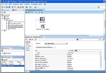
Fig.5. Explore Data function run on sample Insurance table
The Output tab produces a list of all the columns (names and data type) in the data source. The Histogram tab lists the default maximum number (10) of bins (Categorical, Data and Numerical Bins) used for creating histograms. The Sample tab specifies whether all data should be selected for analysis or a percent of the original data should be sampled and used. By default a sampling size of 60% is used. The Statistics (Fig. 6)
IJSER © 2013 http://www.ijser.org
International Journal of Scientific & Engineering Research, Volume 4, Issue 6, June-2013 532
ISSN 2229-5518
produced as a result of applying the explore data function are:
• Attribute name
• Data type
• Histogram
• No. of distinct values
• Mode (for character values)
Minimum, maximum, average, Standard Deviation, etc. (for
Numeric Values)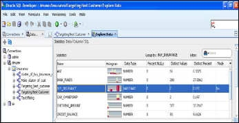
Fig.6. Statistics of Explore Data function
Once it has been ascertained that the data-set can be used to generate some kind of future predictions on the chosen ‘group by’ parameter, we apply the Classification model on the ex- plored data as shown in below Fig. 7.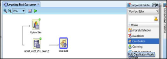
Fig.7. Applying Classification model to IN- SUR_CUST_LTV_SAMPLE
In our case the target field ‘Buy Insurance’ contains binary values (Yes/ No) so the Classification Node ‘Class Build’ builds models using the following four algorithms:
• GLM Classification Models
• SVM Classification Models
• Decision Tree Algorithm
• Naive Bayes
It is important to note that all 4 algorithms are used for a binary target whereas for non-binary targets, the GLM needs to be added explicitly and is not built by default.
Listed below are some important points to be kept in mind while comparing the classification models:
• The training and target data for all models is same.
• All models are tested by default.
• The available data set is randomly split into 2 parts -
50% training data set and 50% test data set which is also
the default split ratio.
• Depending on the Kernel used for creating a model, the information is displayed in the model viewer. The Line- ar Kernel based model displays 3 tabs – Compare, Set- tings and Coefficients. The Gaussian kernel based model displays just 1 tab for Settings.
The results after all Classification algorithms are applied on the data set are as per the below Fig. 8.
Fig.8. Results of Classification Model applied to IN- SUR_CUST_LTV_SAMPLE
The details of each of the Classification algorithm listed in the above Fig. 8. can be viewed by right clicking on the Class Build model, selecting ‘View Models’ and then clicking the appropriate model name from the list. One important thing to note over here is that not all columns in a data source are used while building a model. This happens because some columns may not include any useful information. While in other cases it may happen that a column might contain values of a data type which a given algorithm may not support.
Let us have a look at the details of each of the model one by one:
4.3.1 Decision Tree Model
The classification model generated using the Decision tree algorithm lists the following details for all the nodes:
• Node number
• Prediction
• Support (number of records which satisfy the rule in a given training data set)
• Confidence (if a certain rule has been satisfied then Confidence denotes the likelihood or chances of the predicted outcome)
• No/ Yes Parameters (like, Count, Percentages, and His- togram)
• Split Condition for a node
The leaf nodes contain the final rules generated by the deci- sion tree. The decision tree generated for solving the “Target- ing the Best Customer” problem is as shown in the Fig. 9 be- low:
IJSER © 2013 http://www.ijser.org
International Journal of Scientific & Engineering Research, Volume 4, Issue 6, June-2013 533
ISSN 2229-5518
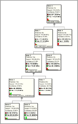
Fig.9. Decision Tree generated for “Targeting the Best Customer”
problem
The 5 leaf nodes (Node 4, 5, 6, 7, 8) denote the five rules generated for solving our problem. The details of each of the rule can be obtained by clicking on each leaf node as shown in Fig. 10.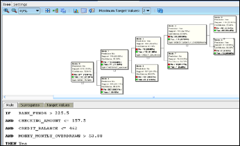
Fig.10. Rule generated for Node 6
All the generated rules are as listed below:
Rule for Node 4
Rule for Node 8
Rule for Node 7
Rule for Node 6
Rule for Node 5
The summary of the Decision Tree generated is as per the be- low Fig. 11: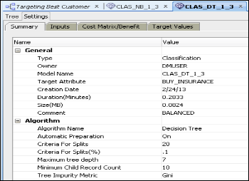
Fig.11. Summary of Decision Tree classification model
IJSER © 2013 http://www.ijser.org
International Journal of Scientific & Engineering Research, Volume 4, Issue 6, June-2013 534
ISSN 2229-5518
The various inputs considered while constructing the Deci- sion tree are as shown in Fig. 12 below.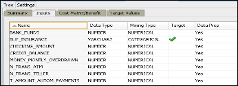
Fig.12. Decision Tree Inputs
The Cost Matrix/ Benefit obtained for the decision tree is as shown belowin Fig. 13: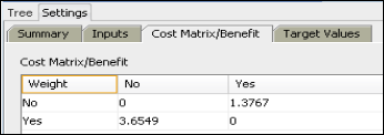
Fig.13. Cost Matrix/ Benefit for Decision Tree model
4.3.2 Support Vector Machine
The SVM model generated for solving the “Targeting the Best Customer” problem is generated using a Linear Kernel and contains the following tabs as shown in figure:
• Coefficients
• Compare
• Settings
The coefficients grid contains the following columns:
Attribute: displays the name of the attribute
Value: contains the value of the attribute. It is a range in
case the attribute is binned
Coefficient: is the probability for the value of the attribute.
Light blue bars denote positive values and red bars denote
negative values as shown in following figure.
This tab allows for a comparison of results for two different target values.
Information about how the model was built is displayed on
the Settings tab. The Summary tab (SVMR) contains the algo-
rithm and model settings. The Inputs tab (SVMC) holds all the
attributes used to build the model and the targets can be
found on the Target Values tab (SVMC). The cost matrix is
displayed on the Cost Matrix/Benefit tab.
4.3.3 Generalized Linear Model
The Generalized Linear Model for solving the “Targeting the Best Customer” problem is as shown in figure below and con- tains 4 tabs – Details, Coefficients, Compare and Settings. The Model details tab lists global metrics (Name and Value of the metric) for the model as a whole. The following metrics (de- fault) are displayed for any GLM. The metrics of high im- portance to us are highlighted in red in the figure. These con- tain: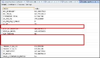
Fig.15. GLM metrics for “Targeting the Right Customer” prob- lem
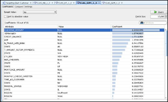
Fig.14. SVM Classification Model for “Targeting the Best Cus- tomer” problem with Positive coefficients
An empty grid indicates the absence of coefficients for target value under consideration. This grid has the below controls:
• Target Value
• Sort By Absolute Value
• Fetch Size
IJSER © 2013
• MODEL_CONVERGED – indicates whether the model converged or not
• NUM_PARAMS – displays the number of parameters
(coefficients, including the intercept)
• NUM_ROWS – displays the number of rows
• PCT_CORRCET – displays the percentage of true (cor- rect) predictions made
• PCT_INCORRCET – displays the percentage of false
(incorrect) predictions made
• PCT_TIED – displays percentage of those cases where probability of both cases is equal (tied)
International Journal of Scientific & Engineering Research, Volume 4, Issue 6, June-2013 535
ISSN 2229-5518
The other tabs for GLM Classification model viewer are similar to the SVM Classification model viewer except for the GLM Compare tab as GLM can only be built for binary classi- fication models.
4.3.4 Naïve Bayes Model
The results generated for the Naïve Bayes model are visually similar to the results obtained for SVM model as blue and red bars with the only difference being in the generated tabs. The various tabs generated for Naïve Bayes model are explained below:
The Probabilities calculated for each feature during the pro- cess of model build are listed under this tab. There is a selec- tion box which allows the user to switch between the two tar- get values – Yes and No. The blue bar in the grid as shown below in Fig. 16 represents positive values for probabilities whereas the red bar represents the negative values for proba- bilities. The tab also facilitates for sorting of displayed proba- bilities and also filtering of features whose probabilities are displayed. For features whose probability value gets close to zero, the bar may not be displayed at all.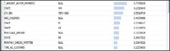
Fig.16. Positive Probability values for features in Naïve Bayes model
By default the probabilities for the value occurring least frequently are displayed.
Using the compare tab results for two different target values can be compared. The selection boxes for Target Value1 and Target Value 2 used for selecting the target values to compare are shown populated with default values. The results of the comparison values selected for target value 1 and target value
2 are displayed in a grid which comprises of the following columns – Attribute (name of the attribute), Value, Propensity for target value, Propensity for target value 2 and histogram bar for both propensities (ranges between 1.0 and -1.0). Pro- pensity is a measure of predictive relationship that a given target value has with a given attribute-value pair. It can be calculated in 2 ways – Propensity for a target value denoted by positive values and propensity against a target value denoted by negative values. The number of records fetched can be changed using the Fetch Sizre variable and the Grid Filter can be used to display specific values. Sort operation can also be performed by click on the grid column headings.
The performance of all the Classification models is compared against each other to determine the best classification model in solving the “Targeting the Right Customer” problem. The Fig.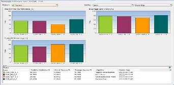
17 below shows the comparative column chart for Predictive Confidence, Average Accuracy and Overall Accuracy meas- ured in % obtained for each classification model.
Fig.17. Comparative Performance Charts generated for classifi- cation models
The table below details the values obtained for each of the model. In all the categories the Decision Tree model generated fares much higher than any other generated model.
Table4. Performance values for generated classification models
Name | Predic- tive Con- fidence % | Over all Ac- curacy % | Av- erage Accura- cy % | Algorithm |
CLAS_S VM_1_3 | 56.5722 | 75.60 48 | 78.2 861 | Support Vec- tor Machine |
CLAS_ NB_1_3 | 54.7736 | 69.95 97 | 77.3 868 | Naïve Bayes |
CLAS_ GLM_1_3 | 39.931 | 80.64 52 | 69.9 655 | Generalized Linear Model |
CLAS_ DT_1_3 | 62.6184 | 81.65 48 | 81.3 092 | Decision Tree |
We find that the decision tree model represented by
CLAS_DT_1_3 provides the best performance amongst all the
4 algorithms in all the 3 performance categories. The formula for calculating the Predictive Confidence for a model is as shown below:
Predictive Confidence =
1 − (Error of Predict)/(Error of naive model) (17)
Error of Predict = 1 − (A1 + A2 + A3)/N (18)
Error of Naive Model = (N − 1)/N (19)
Where, A1 - accuracy for target class 1, A2 - accuracy for
target class 2, etc, and N - number of target classes. The accu- racy for each target class is obtained from the Performance matrix of each model.
IJSER © 2013 http://www.ijser.org
International Journal of Scientific & Engineering Research, Volume 4, Issue 6, June-2013 536
ISSN 2229-5518
For Example, we will calculate the Predictive Confidence of
Decision tree model manually to understand the formula.
Error of predict = 1-(.824658+.801527)/2 = 1-(1.626185/2)
= 1-.8130925 = 0.1869075
Error of naïve model = ((2-1)/2) = 0.50
Predictive confidence = 1-((0.1869075)/0.50) = 1-(.373815)
Predictive Confidence = 0.626185
Fig. 18 below displays the performance matrix for the Deci- sion Tree model displaying the figures for overall and average accuracy. By selecting the appropriate model name from the model drop down box we can view the performance matrix for the other models in a similar fashion.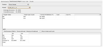
Fig.18. Performance Matrix for Decision Tree Model
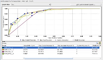
The comparative ROC graph (Fig. 19) of the various Classi- fication models compares the predicted and actual target val- ues. It plots the figures – Max Overall Accuracy, Max Average Accuracy, Custom Accuracy and Model Accuracy, where the X-axis represents the False Positive Fraction and the Y-axis represents the True Positive Fraction.
Fig.19. Comparative ROC curve for all Classification Models
The ROC values generated for all the models are listed as per the below table. In this category too, the results obtained for generated Decision tree model are higher than any other model. However, the generated Generalized Linear Model has results that are in close competition with the obtained ROC values for the Decision tree model.
Table5. ROC Values for different Classification Models
Name | Ar ea Under Curve | Max Overall Accura- cy % | Max Average Accuracy % | C ustom Accu- racy % | Mod el Accu- racy |
CLAS_DT_1_ 3 | 0.8 915 | 82.6 613 | 81.30 92 | 0 | 81.85 48 |
CLAS_GLM_ 1_3 | 0.8 755 | 82.8 629 | 81.19 21 | 0 | 80.64 52 |
CLAS_NB_1_ 3 | 0.8 132 | 73.9 919 | 77.65 03 | 0 | 69.95 97 |
CLAS_SVM_ 1_3 | 0.8 567 | 80.8 468 | 78.86 33 | 0 | 76.41 13 |
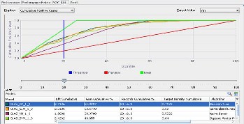
The Lift graph (Fig. 20) displays the trend for Cumulative Positive and Negative cases for the selected target Value (Yes/ No in our case) for all the models.
The red line in the figure below displays the random trend (for randomly generated predictions) and the green line dis- plays the ideal trend values (for model generated predictions).
The blue line indicates the Threshold value. Each line in the graph representing a model displays the rate of convergence of model with the ideal values. The graph presents a compara- tive view of the degree to which the predictions obtained from one classification model are better than randomly-generated predictions. The table below the graph lists the other related Lift values for each model (Decision Tree/ Generalized Linear Model/ Naïve Bayes/ Support Vector Machine) like,
• Lift Cumulative
• Gain Cumulative %
• Records Cumulative %
• Target Density Cumulative
Fig.20. Comparative Lift curve for Cumulative Positive Cases
The table below lists the different Lift values obtained for the various models. Since we had a uniform count of records being used for generating and evaluating each of the models, the values for Records Cumulative % remains same for all the models.
IJSER © 2013 http://www.ijser.org
International Journal of Scientific & Engineering Research, Volume 4, Issue 6, June-2013 537
ISSN 2229-5518
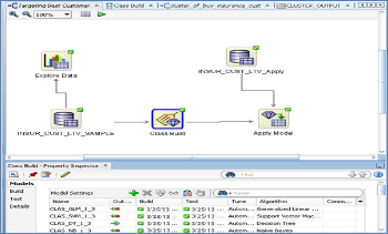
Table6. Lift Values for different Classification Models
Name | Lift Cumu- lative | Gain Cumu- lative % | Records Cumu- lative % | Target Density Cumu- lative | Algorithm |
CLAS_D T_1_3 | 2.7196 | 54.0297 | 20.1613 | 0.7183 | Decision Tree |
CLAS_G LM_1_3 | 2.6125 | 52.6718 | 20.1613 | 0.69 | Generalized Linear Model |
CLAS_N B_1_3 | 1.9036 | 38.3788 | 20.1613 | 0.5028 | Naïve Bayes |
CLAS_SV M_1_3 | 2.4232 | 48.855 | 20.1613 | 0.64 | Support Vec- tor Machine |
In this thesis, we have studied and applied various data min- ing Classification algorithms to solve the Insurance domain problem of “Targeting the Right Customer”, amongst a list of available customers in the Insurance database, for promoting a newly launched Insurance policy. We compared the results obtained from various algorithms on the basis of Performance Matrix, Receiver Operating Characteristics and Lift, and have reached at the following conclusions with respect to the initial defined problem:
• Decision Tree algorithm based model provides the best Average Accuracy (81.31%) , Overall Accuracy (81.65%) and Predictive Confidence (62.61%) to solve the “Targeting the Right Customer” problem at hand.
• The other algorithms follow the performance order - SVM (78.26%), Naïve Bayes (77.38%) and GLM (69.96%) for Average Accuracy; GLM (80.65%), SVM (75.60%) and Naïve Bayes (69.94%) for Overall Accu- racy; and SVM (56.57%), Naïve Bayes (54.77%) and GLM (39.93%) for Predictive Confidence.
• The model based on Decision Tree algorithm also fares the best among the performance Matrix measure by scoring the highest correct predictions percentage of
82.47%.
• Under the ROC figure also, Decision Tree algo- rithm based model obtains the largest Area under the Curve and highest Model Accuracy, followed by GLM, Naïve Bayes and SVM for Area under the Curve and GLM, SVM and Naïve Bayes for Model Accuracy.
• The value for Cumulative Lift is also the highest for
Decision Tree based classification model.
Taking into consideration all the above obtained conclu- sions with respect to the performance of a Classification mod- el, we finally apply the Decision Tree Based model to solve our problem of Targeting the Right Customer for the promo- tion of the newly launched insurance policy (Fig. 21).
Fig.21. Applying Decision Tree Model to the Insurance Customer
Database
In our case, all the result for all performance factors went in favor of Decision Tree based Classification model. This may not be the case for all the other datasets. The performance measuring factors for a given company in the Insurance do- main may differ. Some companies may pay higher weight-age to cost, others to ROC and some others to lift. In such a case, the classification model chosen for application may vary based on the assigned weights or prior conditions set for perfor- mance measures.
Also chances are there, that the chosen model may be a case of Over-fitting when all the data in the database is used only for creating the model. In such cases, the model would give accurate results for data it has already been trained on and not for new data sets.
In our case, we had taken 50% of data for model creation and 50% for testing so the Decision tree model by-passes the fear of being an Over-fitting model.
The classification problem for the Insurance domain has been solved using a Sample Insurance customer database and the performance of the classification algorithms is evaluated on the same data set. However, in a real life scenario, databases are of huge size and contain terabytes of data. Moreover the data sources that feed in data are not limited to hard copies of filled up forms or some system entry but come from a wide domain like the World Wide Web (which comprises of social groups, blogs, twitter posts, etc.). With data input from so many sources, data mining and classification becomes an es- sential part of business operations. It also becomes an im- portant means of gaining competitive intelligence as it would handle huge volumes of data stored in data ware houses and marts and render it in a useful manner [18] by analyzing the same from different perspectives. The new classification sys- tems would be smart enough to suggest hidden and unknown predictions which would ultimately enhance future decision making process.
IJSER © 2013 http://www.ijser.org
International Journal of Scientific & Engineering Research, Volume 4, Issue 6, June-2013 538
ISSN 2229-5518
In such scenarios, technologies like Big Data and Apache Hadoop step in. Almost all big industrial giants have started exploring and implementing the concepts of these new tech- nologies and the ways in which they can utilize the clustering and classification algorithms provided so that new trends, relationships and correlations among the data could be gener- ated (using multidimensional analysis) without incurring the cost of slow operational speeds.
Hadoop is a powerful new technology that is helping com- panies to focus on the most important information in the data collected so that evaluation and understanding of the behavior of potential customers becomes an easy task and this in turn results in capturing of the market. This confidence comes with the huge volumes of data that it can handle and also because of the feature that it can consume unstructured data that comes from sources like blogging sites, social networks and twitter posts.
I am truly indebted to Dr. Udayan Ghose, my guide, for his extended help and encouragement during the making of this thesis. Only through his valuable suggestions and guidance during all the phases of this dissertation could I turn this diffi- cult task into realty. In spite of his busy schedule, he spread his time to give me complete guidance, encouragement and great enthusiasm for successful accomplishment of this disser- tation whenever I needed.
I would also like to express a great sense of gratitude and special thanks to staff of GGSIPU library, without whose co- operation and honest help this study might have not been completed. Above all it is the almighty God who is the one who remains with me in all I do.
Fig.1. Classification ......................................................... 3
Fig.2. Confusion Matrix for a Binary Classification Model….
............................................................................................ 4
Fig.3. Sample Decision Tree (Binary classification) for ‘Target- ing the Right Customer’………………….……............6
Fig.4. Multiple Classifications........................................ 6
Fig.5. Explore Data function run on sample Insurance table 12
Fig.6. Statistics of Explore Data function.................... 12
Fig.7. Applying Classification model to IN- SUR_CUST_LTV_SAMPLE.......................................... 12
Fig.8. Results of Classification Model applied to IN- SUR_CUST_LTV_SAMPLE.......................................... 12
Fig.10. Rule generated for Node 6............................... 13
Fig.11. Summary of Decision Tree classification model 14
Fig.12. Decision Tree Inputs......................................... 14
Fig.13. Cost Matrix/ Benefit for Decision Tree model14
Fig.14. SVM Classification Model for “Targeting the Best Cus- tomer” problem with Positive coefficients................. 14
Fig.15. GLM metrics for “Targeting the Right Customer” prob- lem ................................................................................... 15
Fig.16. Positive Probability values for features in Naïve Bayes model .............................................................................. 15
Fig.17. Comparative Performance Charts generated for classi- fication models............................................................... 16
Fig.18. Performance Matrix for Decision Tree Model16
Fig.19. Comparative ROC curve for all Classification Models
.......................................................................................... 16
Fig.20. Comparative Lift curve for Cumulative Positive Cases
.......................................................................................... 17
Fig.21. Applying Decision Tree Model to the Insurance Cus-
tomer Database .............................................................. 18
Table1. Confusion Matrix……………………………10
Table2. Cost Matrix ....................................................... 11
Table3. INSUR_CUST_LTV_SAMPLE ....................... 11
Table4. Performance values for generated classification models
.......................................................................................... 16
Table5. ROC Values for different Classification Models
.......................................................................................... 17
Table6. Lift Values for different Classification Mod- els………………………………………………..17
[1] Charles Nyce “Predictive Analysis White Paper” American Institute for CPCU/ Insurance Institute of America
[2] Debahuti Mishra, Asit Kumar Das, Mausumi and Sashikala Mishra
“Predictive Data Mining: Promising Future and Applications” Int. J. of Computer and Communication Technology, Vol. 2, No. 1, 2010
[3] Hugh J. Watson, University of Georgia, Barbara H. Wixom, Universi-
ty of Virginia “The Current State of Business Intelligence” IEEE Com- puter Society
[4] Ross Maciejewski, Ryan Hafen, Stephen Rudolph, Stephen G. Larew,
Michael A. Mitchell, William S. Cleveland, and David S. Ebert, “Forecasting Hotspots—A Predictive Analytics Approach” IEEE
[5] Roosevelt C. Mosley Jr., “Social Media Analytics: Data Mining Ap- plied to Insurance Twitter Posts” FCAS, MAAA, Casualty Actuarial Society E-Forum, Winter 2012-Volume 2
[6] Cheu Eng Yeow “Nomograms Visualization of Naïve Bayes Classifi- cation on Liver Disorders Data” School of Computer Engneering, Nanyang Technological University
[7] Christos Tjortjis and John Keane “T3: A Classification Algorithm for Data Mining” Department of Computation, UMIST, Manchester, M60 1QD, UK
[8] Tan, Steinbach, Kumar “Introduction to Data Mining” Addison Wes- ley, 2006
[9] Oracle SQL Developer Release 3 Feature List http://www.oracle.com/technetwork/developer-tools/sql- developer/rel3-featurelist-ea-189447.html
[10] SQLDeveloper3.0Datasheet-350339
IJSER © 2013 http://www.ijser.org
International Journal of Scientific & Engineering Research, Volume 4, Issue 6, June-2013 539
ISSN 2229-5518
http://www.oracle.com/technetwork/developer-tools/sql- developer/sqldeveloper30datasheet-350339.pdf
[11] Oracle® Data Mining Concepts 11g Release 1 (11.1) Part Number B28129
http://docs.oracle.com/cd/B28359_01/datamine.111/b28129/
[12] A.K. JAIN Michigan State University, M.N. MURTY Indian Institute of Science AND P.J. FLYNN The Ohio State University “Data Clus- tering: A Review” ACM Computing Surveys, Vol. 31, No. 3, September
1999
[13] David G. Sullivan, “Data Mining IV: Preparing the Data” Ph.D. Com- puter Science, Boston University, Spring 2013
[14] Mark Tranmer, Mark Elliot “Binary Logistic Regression” Cathie
Marsh Centre for Census and Survey Research
[15] LOWES1 “Predictive Analytics Customer Experiences” Accenture 2010
Global Consumer Survey, published February 8, 2011
[16] Eric Siegel “Predictive Analytics: The Power to Predict Who Will Click, Buy, Lie, or Die” http://www.predictiveanalyticsworld.com/book/
[17] Predictive Analytics - Wikipedia, the free encyclopedia,
http://en.wikipedia.org/wiki/Predictive_analytics
[18] Palak Gupta, “Role of Data Warehousing and Data Mining Technolo- gy in Business Intelligence” Research Journal of Computer Systems En- gineering, Vol 03, Issue 01; January-April 2012
[19] Neelamadhab Padhy, Dr. Pragnyaban Mishra, Rasmita Panigrahi “The Survey of Data Mining Applications And Feature Scope” Inter- national Journal of Computer Science, Engineering and Information Technology (IJCSEIT), Vol.2, No.3, June 2012
[20] Philip Russom “Next generation Data Warehouse Platforms” TDWI
best practices Report, Fourth quarter 2009, www.tdwi.org
[21] Colleen McCue “Data Mining and Predictive Analytics: Battlespace
Awareness for the War on Terrorism”, Defense Intelligence Journal;
13-1&2 (2005), 47-63
[22] Kathleen Ericson, Shrideep Pallickara “On the Performance of High Dimensional Data Clustering and Classification Algorithms” Com- puter Science Department Colorado State University, Fort Collins, CO USA
[23] James Kobielus “Predictive Analytics And Data Mining Solutions, Q1
2010”, The Forrester Wave, February 4, 2010
[24] Hans-Peter Kriegel, Karsten M. Borgwardt, Peer Kröger, Alexey Pryakhin, Matthias Schubert, Arthur Zimek “Future trends in data mining”, Data Min Knowl Disc (2007) 15:87–97 DOI 10.1007/s10618-
007-0067-9
[25] Jaideep Dhok, Vasudeva Varma “Using Pattern Classification for Task Assignment in Map Reduce”, Search and Information Extraction Lab, International Institute of Information Technology, Hyderabad, India,
{jaideep@research.,vv@}iiit.ac.in
IJSER © 2013 http://www.ijser.org