International Journal of Scientific & Engineering Research, Volume 4, Issue 7, July-2013 336
ISSN 2229-5518
Pattern classification for the Handwritten
English vowels with Radial Basis Function
Neural Networks
1Holkar S.R. 2Dr. Manu Pratap Singh
Dept. Of Comp. Sci. Department of Computer Science
Mahatma Gandhi Mahavidyalaya , Institute of Computer & Information Science
Ahmedpur. Dist: Latur(MS) Dr. B.R.Ambedkar
E-mail:shrirangholkar @rediff.com University, Agra -282002
Uttar Pradesh, India
E-mail: manu_p_singh@hotmail.com
Abstract: The purpose of this study is to perform the task of pattern classification for hand written English vowels using radial basis function neural network. This Implementation has been done with five different samples of hand written English vowels. These characters are presented to the neural network for the training. Adjusting the connection strength and network parameters perform the training process in the neural network. By using a simulator program, each algorithm is compared with five data sets of handwritten English language vowels. The 5 trials indicate the significant difference between the two algorithms for the presented data sets. The results
indicate the good convergence for the RBF network.
Key words: Pattern Classification, Radial Basis Function Neural Network, Pattern Recognition.
handwritten character classification task. In this paper we
propose a more suitable and efficient learning method for feed
forward neural networks when neural networks are used as a classifier for the hand written English vowels.
The neural network consists of an input layer of nodes, one or more hidden layers, and an output layer [11]. Each node in the layer has one corresponding node in the next layer, thus creating the stacking effect. The input layer's nodes consists with output functions those deliver data to the first hidden layers nodes. The hidden layer(s) is the processing layer,
where all of the actual computation takes place. Each node in a hidden layer computes a sum based on its input from the previous layer (either the input layer or another hidden layer). The sum is then "compacted" by an output function (sigmoid function), which changes the sum down to more a limited and
manageable range. The output sum from the hidden layers is
IJSER © 2013 http://www.ijser.org
International Journal of Scientific & Engineering Research, Volume 4, Issue 7, July-2013 337
ISSN 2229-5518
passed to the output layer, which exhibits the final network
result. Feed-forward networks may contain any number of hidden layers, but only one input and one output layer. A single-hidden layer network can learn any set of training data that a network with multiple layers can learn [12]. However, a single hidden layer may take longer to train.
In neural networks, the choice of learning algorithm, network topology, weight and bias initialization and input pattern representation are important factors for the network performance in order to accomplish the learning. In particular, the choice of learning algorithm determines the rate of convergence, computational cost and the optimality of the solution. The multi layer feed forward is one of the most widely used neural network architecture. The learning
process for the feed forward network can consider as the
minimization of the specified error (E) that depends on all the free parameters of the network. The most commonly adopted error function is the least mean square error. In the feed forward neural network with J processing units in the output
th
layer and for the pattern, the LMS is given by;
M 2
![]()
E l = ∑ (d l − yl )
being less computationally expensive. However, the
conventional back propagation learning algorithm suffers from short coming, such as slow convergence rate and fixed learning rate. Furthermore it can be stuck to a local minimum of the error.
There are numerous algorithms have been proposed to improve the back propagation learning algorithm. Since, the error surface may have several flat regions; the back propagation algorithm with fixed learning rate may be inefficient. In order to overcome with these problems, vogel et. al. [15] and Jacobs [16] proposed a number of useful heuristic methods, including the dynamic change of the learning rate by a fixed factor and momentum based on the observation of the error signals. Yu et. al. proposed dynamic optimization methods of the learning rate using derivative
information [17]. Several other variations of back propagation
algorithms based on second order methods have been proposed [18-23]. This method generally converges to minima more rapidly than the method based solely on gradient decent method. However, they require an additional storage and the inversion of the second-order derivatives of the error function
with respect to the weights. The storage requirement and
2 j =1
(1.1)
computational cost, increases with the square of the number of weights. Consequently, if a large number of weights are
where l = 1 to L(total number of input-output pattern pairs of training set )
required, the application of the second order methods may be expensive.
Here d j and
y l are the desired and actual outputs
In this paper, we consider the neural networks architecture
which is trained with the gradient descent generalize delta
corresponding to the lth input pattern. Hence, due to the non-
linear nature of E, the minimization of the error function is typically carried out by iterative techniques [13]. Among the various learning algorithms, the back propagation algorithm [14] is one of the most important and widely used algorithms and has been successfully applied in many fields. It is based on the steepest descent gradient and has the advantage of
learning rule for Radial basis function [24] in the single hidden layer for the handwritten English vowels. The rate of convergence and the number of epochs for each pattern are important observation of this study. The simulated results are determined from the number of trails with five sets of handwritten characters of English vowels.
IJSER © 2013 http://www.ijser.org
International Journal of Scientific & Engineering Research, Volume 4, Issue 7, July-2013 338
ISSN 2229-5518
The next section presents the implementation of the neural network architecture with Radial basis function. The experimental results and discussion are presented in section 3. Section 5 contents the conclusion of this paper.
The architecture and training methods of the RBF network are well known [25, 26, 27] well established. The Radial basis function network (RBFN) is a universal approximator with a solid foundation in the conventional approximation theory.
An RBFN is a three layer feed forward network that consists of one input layer, one hidden layer and one output layer as shown in figure (1), each input neuron corresponds to a component of an input vector x. The hidden layer consists of
K neurons and one bias neuron. Each node in the hidden layer
uses an RBF denoted with φ (r ), as its non-linear activation function.
K and M neurons, respectively. φ0 ( x) = 1 , corresponds to the bias.
The hidden layer performs a non-linear transform of the input and the output layer this layer is a linear combiner which maps the nonlinearity into a new space. The biases of the output layer neurons can be modeled by an additional neuron in the hidden layer, which has a constant activation
function φ0 (r ) = 1 . The RBFN can achieve a global optimal solution to the adjustable weights in the minimum MSE range by using the linear optimization method. Thus, for an input pattern x, the output of the jth node of the output layer can define as;
K
y j ( x) = ∑ wkjφk (![]() xi − µk
xi − µk ![]() ) + w0 j
) + w0 j
k =1
(2.1)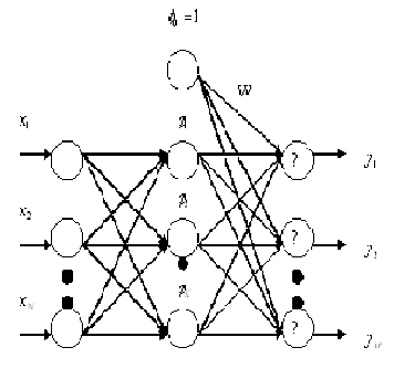
for
j = (1,2,....., , M ) where
y j ( x) is the output of the
j th processing element of the output layer for the RBFN , w is the connection weight from the kth hidden unit to the jth output unit , µk is the prototype or centre of the kth hidden
unit. The Radial Basis Function φ (.) is typically selected as
the Gaussian function that can be represented as:
φk ( xl ) = exp(−
![]()
xl − µk )
2σ 2
for
k = (1,2,....., , K )
(2.2)
and 1 for k = 0 (bias neuron)
Where x is the N- dimensional input vector, µk is the vector determining the centre of the basis function φk and σ k represents the width of the neuron. The weight vector between the input layer and the kth hidden layer neuron can
IJSER © 2013 http://www.ijser.org
International Journal of Scientific & Engineering Research, Volume 4, Issue 7, July-2013 339
ISSN 2229-5518
consider as the centre µk for the feed forward RBF neural network.
Hence, for a set of L pattern pairs{( xl , yl )} , (2.1) can be expressed in the matrix form as
Y = wT φ
(2.3)
where W = [w1 ,..............wm ] is a KxM weight matrix,
in general an optimal procedure so far as the subsequent supervised training is concerned. The difficulty with the unsupervised techniques arises due to the setting up of the basis functions, using density estimation on the input data and takes no consideration for the target labels associated with the data. Thus, it is obvious that to set the parameters of the basis functions for the optimal performance, the target data should include in the training procedure and it reflects
the supervised training. Hence, the basis function parameters
w j = (w0 j ,............wkj )
, φ = [φ0 ,..........φk ] is a K x L
T
for regression can be found by treating the basis function centers and widths along with the second layer weights, as
matrix, φl ,k = [φl ,1 ,..........φl ,k ]
is the output of the hidden
adaptive parameters to be determined by minimization of an
layer for the lth sample, φl ,k = φ (![]() xl − ck
xl − ck ![]() ) ,
) ,
Y = [ y1 , y2, ...... ym ] is a M x L matrix and
y = ( y ..... y )T .
lj l1, lm
The important aspect of the RBFN is the distinction between the rules of the first and second layers weights. It can be seen [28] that, the basis functions can be interpreted in a way, which allows the first layer weights (the parameters governing the basis function), to be determined by unsupervised learning. This leads to the two stage training
error function. The error function has considered in equation (1.1) as the least mean square error (LMS). This error will minimize along the decent gradient of error surface in the weight space between hidden layer and the output layer. The same error will minimize with respect to the Gaussian basis function’s parameter as defined in equation (2.2). Thus, we obtain the expressions for the derivatives of the error function with respect to the weights and basis function parameters for the set of L pattern pairs ( x l , y l ) as; where l = 1 to L.
∂E l
procedure for RBFN. In the first stage the input data set {xn} is used to determine the parameters of the basis functions. The basis functions are then keep fixed while the second – layer weights are found in the second phase of training. There are various techniques have been proposed in the literature for optimizing the basis functions such as unsupervised methods like selection of subsets of
∆w jk = −η1
∆µk = −η2
![]()
∂w jk
∂E l
![]()
∂µk
∂E l
(2.4)
(2.5)
data points [29], orthogonal least square method [30], clustering algorithm [31], Gaussian mixture models [32] and
with the supervised learning method.![]()
and ∆σ k = −η3
∂σ k
M
(2.6)
It has been observed [33] that the use of unsupervised techniques to determine the basis function parameters is not![]()
here, E l = 1 ∑ (d l − yl )2
2 j =1
IJSER © 2013 http://www.ijser.org
International Journal of Scientific & Engineering Research, Volume 4, Issue 7, July-2013 340
ISSN 2229-5518
and yl
K
= ∑ w
![]()
![]()
φ ( xl − µ l )
∂E l
∂E l
∂y l
j
k =1
jk k
k
(2.7)
∆σ k
= −η3
![]()
∂σ k
= −η3
![]()
∂y l
![]()
.
∂σ k
![]()
![]()
2
l l l 2 l l
and φk![]()
( xl − µ l
![]()
) = exp(−
![]()
xl − µ l
)
2σ 2
= −η3![]()
∂E .w
∂y l jk
exp(−
( xi − µki )
2σ 2
xi − µki
) 3
k
![]()
![]()
l l 2 l l 2
Hence, from the equation (2.4) we have,
M K
l l l l
( xi − µki )
xi − µki
∆w = −η
![]()
∂E l
= −η
![]()
∂E l
∂yl
![]()
. j
= −η
![]()
∂E l
![]()
.φ
![]()
l − µ l
or, ∆σ k = η3 ∑∑(d j − y j ).s j ( y j ).wjk .exp(−
j=1 k =1
)
2σ 2 3
jk 1
jk
1 ∂yl
∂w jk
1 ∂yl k x k
(2.10)
So that, we have from equations (2.8), (2.9) & (2.10) the
∂E l
∂s l ( y l )
![]()
( xl − µ l )2
or ∆w jk![]()
= −η1 l l .
∂s ( y )
j j
![]()
∂y l
.exp(−
)
2σ 2
expressions for change in weight vector & basis function
j j j
M K
=η ∑(d l − y l ).sl ( y l ).∑ exp(−
k
![]()
( xl − µ l ) 2
k
parameters to accomplish the learning in supervised way. The
adjustment of the basis function parameters with supervised learning represents a non-linear optimization problem, which
1 j
j =1
j j j
k =1
2σ 2
will typically be computationally intensive and may be prove
So, that
M K
l
l l l
![]()
( xl − µ l )2
to finding local minima of the error function. Thus, for reasonable well-localized RBF, an input will generate a
∆w jk = η1 ∑ ∑ (d j − y j ).s j ( y j ) exp(− σ 2 )
significant activation in a small region and the opportunity of
j =1 k =1
2 k
(2.8)
getting stuck at a local minimum is small. Hence, the training of the network for L pattern pair i.e. ( x l , y l ) will accomplish
∂E l
∂E l
∂y l
Now, from the
equation (2.6) we
in iterative manner with the modification of weight vector and basis function parameters corresponding to each presented
∆µ ki = −η 2
![]()
∂µ ki
= −η 2
![]()
∂y l
![]()
.
∂µ ki
![]()
2
have
pattern vector. The parameters of the network at the mth step of iteration can express as;
l ( l − µ l ) l l
= − η
![]()
∂E .w
xi
. exp(−
ki ).( xi − µki )
M K ( xl − µ l )2
![]()
2 ∂yl jk
![]()
2σ 2 σ 2
w (m) = w
(m −1) +η
(d l − yl ).sl ( yl ).exp(− i ki
j k k
or
jk jk
1 ∑ ∑ j
j=1 k =1
(2.11)
j j j
2σ 2
∆µki =
M K xl − µ l
µki (m) = µki (m −1) +η2 ∑ ∑ (d j − y j ).s j ( y j ).w jk .φk ( xi ).( σ 2 )
![]()
M K ( xl − µ l )2
l
j=1 k =1
l l l
![]()
l i ki
l l l l
i ki k
η2 ∑ ∑ (d j − y j ).s j ( y j )w jk . exp(− σ 2 )
(2.12)
j =1 k =1 2 k
l l
xi − µki
![]()
l l 2
![]()
( ) (2.9)
σ 2
M K
l l l l
l xi − µki
k
Now, from the equation (2.6) we have
σ k (m) = σ k (m − 1) + η3 ∑ ∑ (d j − y j ).s j ( y j ).w jk .φk ( xi ). 3
j=1 k =1 k
(2.13)
IJSER © 2013 http://www.ijser.org
International Journal of Scientific & Engineering Research, Volume 4, Issue 7, July-2013 341
ISSN 2229-5518
where η1 ,η2 &η3 are the coefficient of learning rate. Hence, among the neural network models, RBF network
seems to be quit effective for pattern recognition task such as
handwritten character recognition. Since it is extremely flexible to accommodate various and minute variations in data. Now, in the following subsection we are presenting the simulation designed and implementation details of redial basis function worked as a classifier for the handwritten English vowels recognition problem.
The experiment described in this segment is designed to implement the algorithm for RBF network with decent gradient method.
The task associated to the neural networks in both experiments was to accomplish the training of the
handwritten English language vowels in order to generate the appropriate classification. For this, first we obtained the scanned image of five different types of samples of handwritten English language vowels as shown in figure (2). After collecting these samples, we partitioned an English vowel image in to four equal parts and calculated the density of the pixels, which belong to the central of gravities of these partitioned images of an English vowel. Like this, we will get
4 densities from an image of handwritten English language vowel, which we use to provide the input to the feed forward neural network. We use this procedure of generating input for a feed forward neural network with each sample of English vowel scanned images.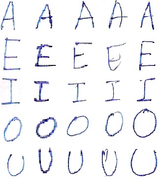
IJSER © 2013 http://www.ijser.org
International Journal of Scientific & Engineering Research, Volume 4, Issue 7, July-2013 342
ISSN 2229-5518
The results presented in this section are demonstrating the implementation of gradient descent learning for RBF network for handwritten English language vowels classification problem. Tables 2 and 3 are representing the results for handwritten English language vowels classification problem performed up to the maximum limit of 50000 iterations.
Language Vowels using decent gradient with RBF network
![]()
English Language Vowels decent gradient with RBF network
Both results contain five different types of handwritten samples for each English vowel character. The training has been performed in such a way that repetition of same input sample for a character can not be happen simultaneously, i.e. if we have trained our network with a input sample of a character then next training can not be happen with the other input sample of the same character. This input sample will appear for training after other samples of other characters training. It can observe from the results of tables that the RBFN has converged for 75 percent cases. The tables are showing some real numbers. These entries represents the error exit in the network after executing the simulation program up to 50000 iterations i.e. up to 50000 iterations the algorithm could not converge for a sample of a hand written English language vowels into the feed forward neural network.
The results described in this paper exhibits the
implementation details for descent gradient learning for radial basis function neural network for the classification of the handwritten English language vowels classification problem.
It has been also observed that the RBF network has also stuck in local minima of error for some of the cases. The reason for
this observation is quite obvious, because there is no
IJSER © 2013 http://www.ijser.org
International Journal of Scientific & Engineering Research, Volume 4, Issue 7, July-2013 343
ISSN 2229-5518
guarantee that RBFNN remains localized after the supervised
learning and the adjustment of the basis function parameters with the supervised learning represents a non-linear optimization, which may lead to the local minimum of the error function. But the considered RBF neural network is well localized and it provides that an input is generating a significant activation in a small region. So that, the opportunity is getting stuck at local minima is small. Thus the number of cases for descent gradient RBF network to trap in local minimum is very low.
1. K. Fukushima and N. Wake, "Handwritten alphanumeric character recognition by the neocognitron," IEEE Trans. on Neural Networks, 2(3) 355-365 (1991).
2. Manish Mangal and Manu Pratap Singh, “Analysis of Classification for the Multidimensional Parity-Bit- Checking Problem with Hybrid Evolutionary Feed-forward Neural Network.” Neurocomputing, Elsevier Science,
70 1511-1524 (2007).
3. D. Aha and R. Bankert, “Cloud classification using error-correcting output codes”, Artificial Intelligence Applications: Natural Resources, Agriculture, and Environmental Science, 11(1) 13-28 (1997).
4. Y.L. Murphey, Y. Luo, “Feature extraction for a multiple
pattern classification neural network system”, IEEE International Conference on Pattern Recognition, (2002).
5. L. Bruzzone, D. F. Prieto and S. B. Serpico, “A neural- statistical approach to multitemporal and multisource remote-sensing image classification”, IEEE Trans. Geosci. Remote Sensing, 37 1350-1359 (1999).
6. J.N. Hwang, S.Y. Kung, M. Niranjan, and J.C.
Principe, “The past, present, and future of neural
networks for signal processing'', IEEE Signal Processing
Magazine, 14(6) 28-48 (1997).
7. C. Lee and D. A. Landgrebe, “Decision boundary feature extraction for neural networks,” IEEE Trans. Neural Networks, 8(1) 75–83 (1997).
8. C. Apte, et al., "Automated Learning of Decision Rules for Text Categorization", ACM Transactions for Information Systems, 12 233-251 (1994).
9. Manish Mangal and Manu Pratap Singh, “ Handwritten English Vowels Recognition using Hybrid evolutionary Feed-Forward Neural Network”, Malaysian Journal of Computer Science, 19(2) 169 –187 (2006).
10. Y. Even-Zohar and D. Roth, “A sequential model for
multi class classification”, In EMNLP-2001, the SIGDAT. Conference on Empirical Methods in Natural Language Processing, 10-19 (2001).
11. Martin M. Anthony, Peter Bartlett, “Learning in Neural Networks: Theoretical Foundations”, Cambridge University Press, New York, NY, (1999).
12. M. Wright, “Designing neural networks commands skill and savvy”, EDN, 36(25), 86-87 (1991).
13. J. Go, G. Han, H. Kim and C. Lee, “Multigradient: A
New Neural Network Learning Algorithm for Pattern Classification”, IEEE Trans. Geoscience and Remote Sensing, 39(5) 986-993 (2001).
14. S. Haykin, “Neural Networks”, A Comprehensive Foundation, Second Edition, Prentice-Hall, Inc., New Jersey, (1999).
15. T. P. Vogl, J. K. Mangis, W. T. Zink, A. K. Rigler, D. L.
Alkon "Accelerating the Convergence of the Back Propagation Method”, Biol. Cybernetics, 59 257-263 (1988)
16. R. A. Jacobs, “Increased Rates of Convergence through
Learning Rate Adaptation”, Neural Networks, 1 295-
307 (1988).
IJSER © 2013 http://www.ijser.org
International Journal of Scientific & Engineering Research, Volume 4, Issue 7, July-2013 344
ISSN 2229-5518
17. X.H. Yu, G.A. Chen, and S.X. Cheng, “Dynamic
learning rate optimization of the backpropagation algorithm”, IEEE Trans. Neural Network, 6 669 - 677 (1995).
18. Stanislaw Osowski, Piotr Bojarczak, Maciej Stodolski, “Fast Second Order Learning Algorithm for Feedforward Multilayer Neural Networks and its Applications”, Neural Networks, 9(9) 1583-1596 (1996).
19. R. Battiti , "First- and Second-Order Methods for Learning: Between Steepest Descent and Newton's Method". Computing: archives for informatics and numerical computation, 4(2) 141-166 (1992).
20. S. Becker, & Y. Le Cun, “Improving the convergence of
the back-propagation learning with second order methods”, In D. S. Touretzky, G. E. Hinton, & T. J. Sejnowski (Eds.), Proceedings of the Connectionist Models Summer School. San Mateo, CA: Morgan Kaufmann,
29-37(1988).
21. M. F. Moller, “A Scaled Conjugate Gradient Algorithm for Fast Supervised learning”, Neural Networks, 6 525-
533(1993).
22. M.T. Hagan, and M. Menhaj, "Training feed-forward networks with the Marquardt algorithm", IEEE Transactions on Neural Networks, 5(6) 989-993(1999).
23. P. Christenson, A.Maurer & G.E.Miner, “handwritten recognition by neural network”, http://csci.mrs.umn.edu/UMMCSciWiki/pub/CSci455
5s04/InsertTeamNameHere/ handwritten.pdf, (2005).
24. M. J. D. Powell, “Radial basis functions for multivariable interpolation: A review”, in Algorithms for Approximation of Functions and Data, J. C. Mason, M. G. Cox, Eds.
Oxford, U.K.: Oxford Univ. Press, 143-167 (1987).
25. T. Poggio, and F. Girosi, “Regularization algorithms for
learning that are equivalent to multilayer networks”,
Science, 247 978-982 (1990b).
26. M. T. Musavi , W. Ahmed , K. H. Chan , K. B. Faris , D. M. Hummels, “On the training of radial basis function classifiers”, Neural Networks, 5(4) 595-603 (1992).
27. W. P. Vogt, “Dictionary of Statistics and Methodology: A Nontechnical Guide for the Social Sciences”, Thousand Oaks: Sage (1993).
28. S. Haykin, “Neural Networks”, Macmillan College
Publishing Company, Inc, New York (1994).
29. D. S. Broomhead and D. Lowe, "Multivariable functional interpolation and adaptive networks", Complex Syst, 2 321-355(1988).
30. M.A. Kraaijveld and R.P.W. Duin, “Generalization capabilities of minimal kernel-based networks”, Proc. Int. Joint Conf. on Neural Networks (Seattle, WA, July 8-12), IEEE, Piscataway, U.S.A., I-843 - I-848(1991).
31. S. Chen, C. F. N. Cowan, and P. M. Grant, “Orthogonal least squares learning algorithm for radial basis function networks”, IEEE Transactions on Neural Networks, ISSN
1045-9227, 2 (2) 302-309(1991).
32. C. M. Bishop, “Novelty detection and neural network validation”, IEEE Proceedings: Vision, Image and Signal Processing. Special issue on applications of neural networks, 141 (4), 217–222(1994b).
33. C. M. Bishop. “Neural Networks for Pattern Recognition”, Oxford University Press, Oxford, New York, (1995).
IJSER © 2013 http://www.ijser.org