𝑢 = 𝜋 𝑥
International Journal of Scientific & Engineering Research, Volume 6, Issue 1, January-2015 606
ISSN 2229-5518
Optimum and Quasi Optimum Adaptive Planar
Arrays Design Using Evolutionary Algorithms
Marian Farouk Mikhail, Mohamed S. El-Mahallawy, Mohamed A. Aboul-Dahab
—————————— ——————————
owadays,adaptive array antennas play an important role in improving signal quality in the wireless communica- tions by keeping the main beam and imposing nulls in
the directions of interfering signals [1]. To reach optimum weight coefficients of array elements adaptively, a variety of algorithms were devised, amongst of which are the evolution- ary algorithms [2], [3]. In evolutionary algorithm, a fitness function is formed to match a required design criterion, and relevant optimum weights are reached via variation and selec- tion operation [2], [3], [4]. Two of the mostly used evolution- ary algorithms in the design of adaptive antenna arrays are the Genetic Algorithm (GA) and particle swarm optimization (PSO) algorithm [5]. In [6], the GA was utilized to seek opti- mum weights linked to antenna elements that result in the reduction of side lobe level.
The GA was used for the synthesis of antenna array radia- tion pattern in adaptive beam forming [7]. In [5],[8]the design of non uniformly spaced linear antenna arrays using PSO al- gorithm was presented for the purpose of reaching a desired radiation pattern while improving the performance of these arrays in terms of side lobe levels.Another approach was pre- sented in [2], where the synthesis of linear antenna array using PSO algorithm was carried out to reach optimum ampli- tude excitations for performance improvement in the sense of minimum side lobe level (SLL) and null control with periodic spacing between the elements.
Due to the usage of adaptive planar array in a variety of
————————————————
applications such as tracking radars, search radars, remote sensing and communication systems, and due to additional variables which can be used to control and shape the array pattern ,a lot of research have been developed to improve the performance of these arrays[9]. In [3], planar array synthesis using Chebytshev’s method and GA was proposed to control the amplitude and phase of signals of array elements for the purpose of placing nulls at the directions of the interfering sources and placing the main beam in the direction of the de- sired signal. Another approach was devised using the GA to seek the optimum weight coefficients of the array elements to achieve a minimum SLL with narrower beam width. The re- sults were compared with synthesized pattern using Gaussian, Kaiser, Hamming and Blackman weights coefficients where a significant improvement had been achieved [4]. The PSO had been utilized to control Signal-to-Interference-plus-Noise Ra- tio and to find the set of weights that configure a rectangular array to effectively maximize the power towards a desired direction and avoid direction of interferers [10].
A comparison between the GA and the PSO for the design of linear and planar antennas arrays with uniformly spaced elements for the purpose of side lobe reduction and main beam width constraints had been carried in [11]. The weights adjustment via amplitude only and amplitude plus phase had been investigated. The results showed that an appreciable re- duction of the order of the first SLL that had been attained in comparison with the case of uniform arrays. Also, the results showed that PSO with adaptive scheme had a better perfor- mance than GA due to its simplicity in implementation and minor computing time. [11]
In this paper a design procedure for an optimum adaptive beamforming planar arrays is introduced by changing the ar- ray weight coefficients and the spacing between array ele- ments with multiple constrains using the GA and PSO algo- rithms .These constrains deal with the array parameters (which are the first null beam width, the first SLL, and a null imposed at certain direction) and with the evolutionary algo-
IJSER © 2015
International Journal of Scientific & Engineering Research, Volume 6, Issue 1, January-2015 607
ISSN 2229-5518
rithms(the weights of the cost function, the limits of array weight coefficients and limits of the spacing between array elements). For the ease of implementation, quasi-optimum weights are chosen, where an additional constraint to the op- timization cost function is also imposed.
This paper is organized as follows. In section 2, problem formulation will be discussed. In section 3, a brief description of the utilized optimization techniques, namely the GA and PSO is given. The optimum and quasi optimum arrays are described in sections 4 and 5 respectively. Computer simula- tion results and discussions are given in section 6, and the pa-
where AF(null)i is the value of the designed array factor at the particular null position, AFmax is the maximum value of the array factor, Q is the SLL of the desired array in dB at peak point θk & ϕk , δ is the desired value of the SLL in dB of the uniform array, FNBWcomputed is the computed first null beam width of the designed array , the value of the FNBW(an,am=1) of the uniform array , C1 , C2 & C3 are weighting coefficients used to control the relative importance of each term of Equa- tion (2) and H is defined as
1 (𝑄 − 𝛿 ) > 0
per is concluded in section 7.
𝐻 = �
0 (𝑄 − 𝛿 ≤ 0
� (3)
For a planar array composed of even number of elements (2M*2N) symmetrically placed over along the x-z plane, as shown in Fig.1. The planar array factor is given by [12], [13]
where the side lobes whose peaks exceed the threshold δ must be suppressed. The solution of the optimization problem will yield the required weight coefficients (amplitudes) as well as the inter- element spacing in the dimensions of the array.
𝐴𝐴 = 4 ∑𝑀
where
𝑁
𝑛=1
𝑎𝑚 ∗ 𝑎𝑛 ∗ 𝑐𝑐𝑐[(2𝑚 − 1)𝑢] ∗ 𝑐𝑐𝑐[(2𝑛 − 1)𝑣]
![]()
𝑢 = 𝜋 𝑥
λ 𝑚
![]()
𝑐𝑠𝑛𝑠𝑐𝑐𝑐𝑠 & 𝑣 = 𝜋 𝑧 𝑐𝑐𝑐𝑠 (1)
λ 𝑛
It is based on principle of the evolution of the natural species
introduced by Charles Darwin [14]. The optimization process
in the (GA) is based upon the following procedure [15]:
1- Creating an initial random population of weights of
elements and inter distance between elements.
2- Evaluation of population based on the fitness function
of (2).
3- Some values (chromosomes) are selected as a parent
by a selection technique (roulette wheel-tournament).
4- Offspring and Mutation can be generated from select-
ed parents.
5- The process will continues until the termination con-
dition is achieved.
Unlike GAs, the PSO is based upon the cooperation among the
Fig. 1.planar array composed (2M*2N) elements symmetrically
placed over an along the X-Z plane.
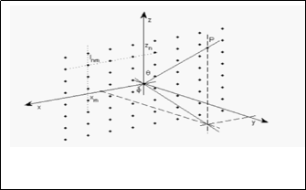
where am , an are the amplitude excitations, xm is the position of the mth element and zn is the position of the nth element.
It is required to design this array in such a way that the fol-
lowing objectives are achieved:
1- A null to be imposed at certain direction.
2- The Fisrt null beam width to be kept unchanged with
respect to uniform array.
3- First SLL to be reduced below that of a uniform array.
These objectives represent constraints that are imposed on
the design procedure of the array. In this respect, a cost func-
tion (CF) is developed to be minimized. An expression for the
cost function will contain three additive terms inspired from
[1] as
individuals rather than their competition. Moreover, it is easi- er to calibrate and to control the parameters of the PSO over the GA [16].
In PSO, the optimization process proceeds as follows[17]:
1- Each particle is initialized with a random position and velocity.
2- Each particle is then evaluated for fitness value of (2).
3- Each time a fitness value is calculated, it is compared
against the previous best fitness value of the particle
and the previous best fitness value of the whole
swarm, and the personal best (pbest) and global best
positions (gbest ) are updated where appropriate.
4- The process is repeated until a stopping criterion is
met.
The far field pattern of an array is controlled by many factors.
|𝐴𝐴(𝑛𝑢𝑛𝑛𝑖 )|
𝐻 ∗ (𝑄 − 𝛿)
In addition to the geometrical configuration of the overall ar-![]()
![]()
𝐶𝐴 = 𝐶1 ∗ (|𝐴𝐴(𝑚𝑎𝑥)|) +𝐶2 ∗ �
(𝛿 ) � +𝐶3
ray, there are the relative displacement between elements, ex-![]()
∗ �𝐴𝐹𝐹𝐹𝐶𝑜𝑚𝑝𝑢𝑡𝑒𝑑 − 𝐴𝐹𝐹𝐹𝑎𝑛,𝑎𝑚=1�
�𝐴𝐹𝐹𝐹𝑎𝑛,𝑎𝑚=1�
� (2)
citation amplitudes of individual elements, excitation phase of
individual elements, and far field pattern of the individual
elements [5]. In this paper, inter-spacing between elements, excitation amplitude of individual elements will be optimized
IJSER © 2015 http://www.ijser.org
International Journal of Scientific & Engineering Research, Volume 6, Issue 1, January-2015 608
ISSN 2229-5518
to achieve the required first null beam width, lower value of the first SLL and a null that is imposed at certain direction.
The weighting coefficients C1 , C2 and C3 of the cost func- tion are selected according to there relative importance of the imposed constraint. In the proposed design, we emphasize on the superiority of the imposed null as well as the first null beamwidth. For this reason, the ratio of the coefficients is tak- en to be 1: 3: 3 respectively. In order to obtain reasonable val- ues for the optimum weight coefficients of array elements, as well as optimum inter element distances of the array, some constraints need to be imposed on the cost function. Moreo- ver, appropriate values have to be selected for the initiation of the optimization process. The following is a proposed con- straint on the weight coefficients of array elements:
0.5 ≤ 𝑤𝑖,𝑗 ≤ 1 i=1,2,…M , j= 1,2, … N (4)
As far as the inter element distances are concerned, the follow-
ing constraint is proposed
0.25λ ≤ 𝑑𝑥 , 𝑑𝑧 ≤ 0.5λ (5)
The upper bound is necessary to avoid the presence of grating
lobes in the visible range of the array. It is worth mentioning
that the above constraints are applied to both E-plane pattern
and H- plane pattern of the array.
The optimum values of the weights and distances can take any value within the imposed bounds. For ease of implementation of the array, it is more reasonable to have a number of dis- crete, rather than continuous values of the optimum values. For this reason, the optimum weight coefficients are approxi- mated to two discrete values, namely 0.5 and 1.0. As far as the inter element distances are concerned, three discrete values are selected, namely 0.3λ, 0.4λ and 0.5λ. Actually, the approx- imated values will not yield the required optimum array per- formance. We shall rather have a quasi optimum array. The approximated values of the weights and inter element dis- tances are derived from the optimum weights that are ob- tained from using either the GA or the PSO algorithm. The performance of the quasi optimum arrays is investigated in the next section to have some insight on the limitations and tolerances in their performances.
The case of a planar array composed of 12 x 12 elements is considered. The array is placed symmetrically on x-z plane, and is assumed to be uniform in its initial condition with weight coefficients to be unity and inter element distances in both directions to be 0.5 λ.The constraints imposed on the ar- ray are as follows:
• First null beamwidth (FNBW) = 0.334 radians (same as that of the uniform array)
zation problem has been developed using MATLAB 14 soft- ware package, where the results of 25 optimization runs using the GA and PSO algorithms have been obtained. PSO &GA parameters are empirically chosen to achieve the best results in our simulation. The following are the parameters utilized in the simulation process with either GA or PSO algorithm
Table 1: GA and PSO Parameters![]()
Algorithm Parameters Values
GA | Population size | 100 |
Generations No. | 100 | |
Weights upper limit | 1.0 | |
Weights lower limit | 0.5 | |
Inter elements distances upper limit | 0.5 | |
Inter elements distances lower limit | 0.25 | |
Crossover rate | 0.8 | |
Mutation rate | 0.01 | |
PSO | Particles swarm | 100 |
Iterations No. | 100 | |
Weights upper limit | 1.0 | |
Weights lower limit | 0.5 | |
Inter elements distances upper limit | 0.5 | |
Inter elements distances lower limit | 0.25 |
![]()
![]()
The maximum and minimum values of the FNBW, im- posed null and first SLL in both x-y and y-z planes in the de- signed of optimum and quasi optimum arrays using the GA and the PSO algorithms are shown in Table2. It is clear from the results in the case of optimum array, that PSO gives near- ly the same FNBW as in the imposed constraint rather than the case of GA. The null imposed at the required angles is deeper in the case of PSO than that of the case of GA. However, a con- siderable reduction in the level of the first SLL has been achieved in the case of the PSO than that in the case of GA.In the case of quasi optimum array, the values of the FNBW are not so far from the imposed value. The level of the imposed null is not so deep, and the first SLL in some runs are higher than that of the imposed constraint.
Table 2: Maximum and minimum values of FNBW, null depth and first SLL![]()
.
Array Optimum Array Quasi Optimum
Array
• Deep nulls to appear at angles θn = ϕn =54.43o ( the
plane
Algorithm
PSO GA PSO GA
angles at of the 3rd side lobe in the uniform array) and to be less than -40dB.
• A reduction of the first SLL (at angles θ1L = ϕ1L =76.2o )
below that of the uniform array.
To investigate the performance of the optimum and quasi
optimum planar arrays, a computer simulation for the optimi-
constraint
y-z FNBWmax(rad) 0.347 0.340 0.360 0.360
FNBWmin (rad) 0.340 0.340 0.340 0.340
x-y FNBWmax(rad) 0.347 0.340 0.354 0.360
FNBW min (rad) 0.340 0.326 0.340 0.340
y-z Null level max
(dB) -122.950 -98.231 -22.965 -43.186
IJSER © 2015 http://www.ijser.org
International Journal of Scientific & Engineering Research, Volume 6, Issue 1, January-2015 609
![]()
ISSN 2229-5518
Null level min
(dB) -45.367 -50.920 -13.946 -13.538
x-y Null level max
(dB) -108.554 -101.188 -30.971 -37.005
Null level min
3rdNull level y-z x-y
-78.258
±57.11%
-78.938
±40.08%
-20.133
±30.7%
-23.093
![]()
±34.12%
-20.57
-75.211
±32.3%
-71.841
±42.08%
-20.51
±110.56%
-23.16
±59.78%
![]()
-13.902
(dB) -47.299 -41.609 -18.445 -10.984
y-z SLL max (dB) -30.395 -20.127 -31.803 -21.372
First SLL
y-z -27.342
±41.51%
±54.639% -15.719
±96.56%
±53.73%
SLL min (dB) -15.993 -13.289 -10.233 -8.611
x-y SLL max (dB) -35.307 -27.389 -36.69 -29.195
![]()
SLL min (dB) -18.190 -11.453 -18.963 -9.1203
x-y
-28.604
![]()
±36.41%
-23.86
±53.74%
-18.053
±51.71%
-17.235
±69.39%
The stability of the deigned performance of the optimum and quasi optimum planar arrays are investigated by monitor- ing the average values of the 25 optimization runs that have been carried out for both cases of PSO and GA. The deviations from the average values are also monitored for both cases. Table3 illustrates the average values of the FNBW, null depth and first SLL as well as the deviations from the average. It is clear that the FNBW in both optimum and quasi optimum arrays have been achieved with satisfactorily percentage of deviation using both algorithms. The first SLL constraint has been achieved in the optimum array using both algorithms although the percentage deviation is relatively high. It is nota- ble that the PSO has a superior performance since its percent-
age deviation is lower than that of the GA algorithm. As for
the quasi optimum array, the first SLL constraint has been
marginally achieved, but the percentage deviation is consider-
ably high. As far as the deep null is concerned, the optimum
array has satisfactorily achieved the required constraint alt-
hough the percentage deviation is considerably high. Howev-
er, the quasi optimum array has not achieved the required
constraint, in addition to the remarkable high deviation per- centage.
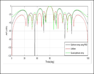
The array factor using best optimized and quasi optimized values of weight coefficients as well as inter element distances are shown in Fig. 2, Fig.3 for the x-y and y-z planes for the case of PSO algorithm. It is clear from these figures that the array factors for the optimum and quasi optimum arrays are very close to each other except at the location of the imposed null where the quasi optimum array has not achieved this constraint.![]()
![]()
Table 3: The average and maximum deviation values of FNBW, null depth and first SLL for optimum and quasi optimum arrays using PSO and GA algorithms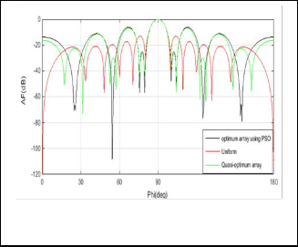
Fig. 4, Fig.5 illustrate the array factors using best optimized and quasi optimized values of the weight coefficients and inter element distances for the x-y and y-z planes for the optimum and quasi arrays for the case of the GA algorithm. It is clear from these figures that the array factors for the optimum and quasi optimum arrays are far from each other except at the location of the main lobe.
Fig. 2.x-y plane for planar array factor (Optimum array using
PSO, uniform and Quazi-optimum array)
Fig. 3.y-z plane for planar array factor (Optimum array using
PSO, uniform and Quazi-optimum array)
IJSER © 2015 http://www.ijser.org
International Journal of Scientific & Engineering Research, Volume 6, Issue 1, January-2015 610
ISSN 2229-5518
the optimum arrays have achieved the imposed constraints. However, the performance of quasi optimum arrays has been found partially satisfactory. It is worth noting that use of PSO has resulted in superior performance over that of the GA in both optimum and quasi optimum arrays.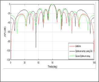
Fig. 4.x-y plane for planar array factor (Optimum array using GA, uniform and Quazi-optimum array)
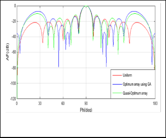
Fig. 5.y-z plane for planar array factor (Optimum array using GA, uniform and Quazi-optimum array)
The design of optimum planar array under certain imposed constraints is presented in this paper. The optimum values of the weigh coefficients as well as the optimum inter element distances have been achieved using two evolutionary algo- rithms, namely the particle swarm optimization (PSO) and the genetic algorithm (GA). A quasi optimum array has been de- vised in both cases by rounding the weight coefficients and inter element distances to a limited number of discrete values. This approach has a practical advantage since it is possible to have certain preset values for the weight coefficients and the inter element distances. The simulation results illustrated that
[1] B. Goswami, D. Mandal , A G. Algorithm For The Level Control Of Nulls
And Side Lobes In Linear Antenna Arrays, Journal of King Saud University
– Computer and Information Sciences vol.. 25, Issue 2, pp. 117–126, July
2013.
[2] L. Pappula, D. Ghosh, Linear Antenna Array Synthesis For Wireless Com- muni cations Using Particle Swarm Optimization, 15 th international confer- ence on advanced communication technology (ICACT2013),pp.780-
783,PyeongChang, January 27 ~ 30, 2013.
[3] A. Hammami, R. Ghayoula and A. Gharsallah 1, Design Of Planar Array Antenna With Chebytshev Method And Genetic Algorithm, Unité de re- cherche ,Circuits et systèmes électroniques HF Faculté des Sciences de Tunis, Campus Universitaire Tunis EL-Manar, 2092, Tunisie .
[4] A.K. Aboul-Seoud, A. K. Mahmoud, and A.Hafez, A Sidelobe Level Reduc- tion (SLL) For Planar Array Antennas, 26th National Radio Science Confer- ence (NRSC2009) ,new cairo,Egypt,pp.1-8, 17-19 march 2009
[5] M. M..Khodier, C. G. Christodoulou, Linear Array Geometry Synthesis With Mininum Side Lobe Level And Null Control Using Particle Swarm Optimi- zation, IEEE Transactions on Anthennas and Propagation, vol. 53, No. 8, pp.2674-2679, August 2005.
[6] P.M. Mainkar, S..S.Ghule, O..S.Ghate, R..N.Ojha, Optimal Side Lobe Reduc- tion Of Linear Nonuniform Array Using Genetic Agorithm, International Journal of Computer Architecture and Mobility (ISSN 2319-9229), vol. 1, Issue 6, April 2013.
[7] S. Shrivastava, K. Cecil ,Performance Analysis Of Linear Antenna Array
Using Genetic Algorithm, International Journal of Engineering and Inno- vative Tech nology (IJEIT) , vol. 2, Issue 5, pp. 84:88 , November 2012.
[8] A. Recioui, J. Optim, Sidelobe Level Reduction In Linear Array Pattern Synthsis Using Particle Swarm Optimization, Springer Science+Business Media, LLC 2011.
[9] C.A.Balanis, Antenna Theory: Analysis and Design, 3rd ed, Wiley&S ons
2005.,pp.349.
[10] V. Zuniga, A. Erdogan, T. Arslan, Control of Adaptive Rectangular Antenna
Arrays Using Particle Swarm Optimization ,2010 Loughborough Antennas
& Propa gation Conference, Loughborough, UK, 8-9 November 2010.
[11] B. Kadri1, M. Brahimi1, I.K. Bousserhane1, M. Bousahla2, F.T. Bendimerad, Patterns Antennas Arrays Synthesis Based On Adaptive Particle Swarm Op- timization and Genetic Algorithms, IJCSI International Journal of Computer Science Issues, vol. 10, Issue 1, No 2, pp.21-26,January 2013,
[12] F. I. Tseng, and D. K. Cheng (1968), Optimum Scannable Planar Arrays With An Invariant Sidelobe Level, Proc. IEEE, vol.. 56, Issue 11 , pp.1771 – 1778, November 68.
[13] P. Nicoletta; K., MajidM; A., Mirko; R., M. Barbin, E .Silvio and G. Chris- todoulou , Christos, Planar Array Synthesis With Minimum Side lobe Level And Null Control Using Particle Swarm Optimization., Microwaves, Radar
& Wireless Communications, 2006. MIKON 2006. pp.1087 –
1090,.may2006,karkow
[14] N. Sivanandam ،S. N. Deepa , Introduction To Genetic Algo- rithms,SpringerBerline Heidelberg 2008,Chapter 2, pp.15.
[15] Randy L. Haupt and Douglas H. Werner,Genetic Algorithms In Electormag- netics, Wiley-ieee 2007.2nd Edition .Chapter 2, pp.29-43.
[16] M. Donelli, R. Azaro, F. G. B. D. Natale, and A. Massa, “An Innovative Com-
IJSER © 2015 http://www.ijser.org
International Journal of Scientific & Engineering Research, Volume 6, Issue 1, January-2015 611
ISSN 2229-5518
putational Approach Based On A Particle Swarm Strategy For Adaptive Phased-Arrays Control,” IEEE Transactions on Antennas and Propaga- tion,vol. 54, no. 3, pp. 888–897, March 2006.
[17] V. Kachitvichyanukul, Comparison Of Three Evolutionary Algorithms:
GA, PSO, and DE, Industrial Engineering& Management Systems vol. 11, no. 3, pp. 215-223, September 2012.
IJSER © 2015 http://www.ijser.org