Optimization of Axial Flow Turbine for Mean-Line Design using Genetic Algorithm

International Journal of Scientific & Engineering Research, Volume 6, Issue 1, January-2015

ISSN 2229-5518

640

——————————  ——————————

he turbine design is a trade-off between aerodynamic, thermal, structural and manufacturing requirements. Hence, optimization plays an important role in the turbine design and development. The future trend in design optimiza- tion is to cover not only aerodynamic performance of turbines, but also creep life and weight of the turbine stage. Life cycle costs and product cycle time are additional, possible criteria during the design optimization process. Starting a new design, basic preliminary design steps calculate the mean dimensions
of the machine.
The mean line design has the largest influence on the final
product. The optimized mean line design greatly reduces the
number of design iterations and the development time. The
optimization methods, strategies for the axial flow turbine are given in [1], [2], [3], [4], [5]. In the mean line design, the
meridional flow path, mean velocity triangles, number of vanes and blades are obtained by ensuring the required life and weight of the turbine stage. The results of the parametric study for the mean line design by considering the conflicting requirements of aerodynamic performance, creep life and weight are discussed in [6].
In general, if a function is defined on the basis of the design variables, depending upon the conditions of the efficiency, life and weight, the process of optimization, i.e the minimization or maximation, depending on the formulation of the fitness function, is to find out the right combination of the design variables, which will yield the best possible design in terms of aerodynamic performance, life and weight of the turbine module.
In the present study the optimization is carried out using the genetic algorithm. The genetic algorithm is a method for solving both constrained and unconstrained optimization problems that is based on natural selection, the process that

————————————————

 S V Ramana Murthy is currently pursuing doctoral degree program in Mechanical engineering in Visvesaraya Technological University, India, E-mail: seepana.ramana@gmail.com.

 S Kishore Kumar is currently Scientist in Gas Turbine Research Estab- lishment, India.

drives biological evolution. The genetic algorithm repeatedly modifies a population of individual solutions. At each step, the genetic algorithm selects individuals at random from the current population to be parents and uses them to produce the children for the next generation. Over successive generations, the population "evolves" toward an optimal solution.
The genetic algorithm is applied to solve a variety of opti- mization problems that are not well suited for standard opti- mization algorithms, including problems in which the objec- tive function is discontinuous, non-differentiable, stochastic, or highly non-linear. The genetic algorithm uses three main types of rules at each step to create the next generation from the current population: a) Selection rules select the individu- als, called parents that contribute to the population at the next generation. b) Crossover rules combine two parents to form children for the next generation. c) Mutation rules apply ran- dom changes to individual parents to form children. The ge- netic algorithm differs from a classical, derivative-based, op- timization algorithm in two main ways. Classical algorithms Generates a single point at each iteration, the sequence of points approaches an optimal solution and Selects the next point in the sequence by a deterministic computation whereas genetic algorithms Generates a population of points at each iteration, the best point in the population approaches an opti- mal solution and Selects the next population by computation which uses random number generators [7], [8], [9].

A computer code is developed for the mean line design of an axial flow turbine to achieve high turbine efficiency by con- sidering aerofoil cooling, castablity, structural aspects and weight. The Turbine mass flow (m), Inlet Total Pressure (P01), Inlet Total Temperature (T01), Power (P) to be produced, the target Total to total isentropic Efficiency(η) are obtained from the engine thermodynamic cycle. The rotational speed of the turbine is fixed by the compressor, because of the adverse pressure gradient in the compressor. The design variables for the mean line design are the flow coefficient(φ), the stage load- ing(ψ) and the turbine exit swirl angle(α3). Besides these, pa-

http://www.ijser.org

International Journal of Scientific & Engineering Research Volume 6, Issue 1, January-2015

641

rameters like the Nozzle Guide vane and blade aspect ratio, Rotor Axial velocity ratio(Ca3/Ca2), NGV Axial velocity ra- tio(Ca1/Ca2), Blade speed ratio for Constant mean (KUm)/ biased design need to be specified based on the type of the turbine. The value of the Nozzle Guide vane loss coefficient is assumed initially.
Using the input parameters the meridional flow path, mean velocity triangles, stress function and reaction are calculated. The losses are estimated using the empirical correlations given in the references [10], [11],[12]. Incidence losses are estimated using the correlations given in the reference [13]. The optimum space-chord ratio and hence the number of blades are estimated using the correlation as explained in [10]. The corresponding aerofoil geometric characteristics are obtained based on the method explained in reference [10],[14].
The output contains the meridional flow path, number of
blades and vanes, mean velocity triangles, blade and vane
mean section geometric parameters, creep life and weight of the turbine stage.
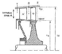
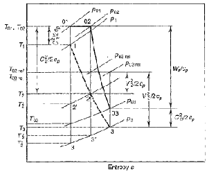
The nomenaclature of the axial stations, the T-s diagram of the turbine stage and velocity triangle parameters are shown in Figures 1, 2 & 3 respectively.

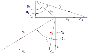
Fig.3. Parameters of the velocity triangle

The mathematical formulation of the meanline design [15],[16],[17],[18] to evaluate the geometrical faeatures and turbine performance is given below.

𝑃 = �� Δ�

𝑃��

�� Δ� = �

𝜔 =

2��

Fig.1. Nomenclature of Axial Stations
Evaluation of the Mean Radius: Hence,

�� ΔT

Ψ =

�2

�� ΔT

U =

Fig.2. T-s diagram of Turbine stage

�

�� = 𝜔

Evaluation of the Pressure Ratio:

http://www.ijser.org

3 3

International Journal of Scientific & Engineering Research Volume 6, Issue 1, January-2015

M = �3

3 �

642

𝜂� −� =

Δ�

� −1

�

Ma3 =

�� 3

�

�01 1 −

𝑃01

𝑃03

Mr3 =

��3

�

𝑃01 =

𝑃03

1 − Δ�

𝜂�01

� −1

�

T03rel = �3 1 +

� − 1

��3 2

�� 2 = �Φ

�� 3

P03rel

� − 1

= 1 +

��3 2

�

� −1

�� 3 = �� 2

�� 2

Calculations at Station 2

Um2 = U

Calculations at Station 3

�� 3 = ��

�� Δ� = � �� 2 �� 2 + �� 3 �� 3

β3 = tan−1

� + �𝜔 3

�� 2 =

�� ∆T − Um3 Cw3

�𝜔 3

= �� 3

��3

�� 3

�� 2

α2 = tan−1

�𝜔 2

�� 2

�3 =

T03 = T01 − Δ�

� 3

α2 = tan−1

�𝜔 2

�� 2

��3

�3 2

�� 2

C =

T3 = T03 − 2�

Vr3 = �� 3 2 + �� 3 + �𝜔 3 2

C2 =

�� 2

��2

P = P01

03 𝑃�. ��𝑖�

Vr3 = �� 2 � 2 � 2

Vr3 = �� 2

+ �� 2 − �� 2 2

P3 = 𝑃03

�3

�03

�

� −1

β = tan−1 � 𝜔 2 − �� 2

−1 �𝜔 2�−� 2�� 2

a3 = ��3

M = �3

3 �3

β2 = tan

T2 = T01 −

�� 2

�2 2

2��2

2��

Ma3 =

�� 3

�3

a2 = ��2

M = �2

2 ��2

Mr3 =

T03rel = �3 1 +

��3

�3

� − 1

��3 2

http://www.ijser.org

M2 =

Ma2 =

�2

�� 2

�

� 2

�2

�

a2 = ��2

International Journal of Scientific & Engineering Research Volume 6, Issue 1, January-2015

�2

643

M2 =

Ma2 =

�2

�� 2

�

Roter outlet blade height,

h = �3

3 2��

Mr2 =

��2

�2

Yr =

𝑃02�� − 𝑃03��

𝑃03�� − 𝑃3

ℎ2 + ℎ3 2

𝑃01 − 𝑃02

Cx � =

ℎ � �

Ys = 𝑃

− 𝑃

�

ℎ3 ℎ2

02 2

𝑃01

�� 3 − 2 − �� 2 − 2

Rotor Hub Flare Angle = tan−1

��

P02 =

1 + �� 1 −

�2

�02

�

� −1

Rotor Tip Flare Angle = tan−1

�� 3 +

ℎ3 ℎ2

2 − �� 2 + 2

��

P2 =

𝑃02

1 + � − 1

�� 2

�

� −1

Calculations at Station 1

C = � �� 1

a1 � 2 �� 2

�� 1

Areas at Station 2 and 3

C2 =

cos �1

�1 2

ρ2 =

𝑃2

��2

T1 = T01 − 2�

a1 = ��1

Rotor inlet area,

�

A2 = � �

�1

M1 =

2 � 2

�

�1 � −1

Rotor inlet blade height,

h = �2

2 2��

𝑃3

P1 = 𝑃01

ρ1 =

�01

𝑃1

��1

ρ3 = ��

Rotor outlet area,
Stator inlet area,

�

A1 = � �

1 � 1

Stator inlet blade height,

h = �1

1 2��

ℎ1 + ℎ2 2

http://www.ij Cx � =

ℎ ��

International Jo�ur1nal of Scientific & Engineering Research Volume 6, Issue 1, January-2015

h1 = 2��

644

Cx � =

ℎ1 + ℎ2 2

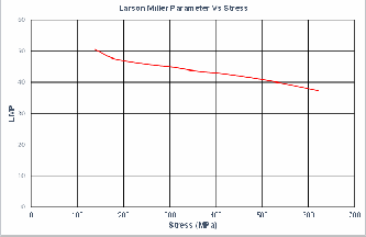
Further the creep life is estimated from the Larson Miller
parameter [19], Tmetal and σc shown in Figure 4 and the rela-

ℎ ��

tion:

ℎ2 ℎ1

Stator Hub Flare Angle = tan−1

�� − 2 − �� − 2

��

ℎ2

�� +

ℎ1

− �� +

Stator Tip Flare Angle = tan−1

2 2

��

�

Zweifel Loading = 2

�

��2 �2 tan �2 + tan �1

With these mean geometrical and flow parameters, the losses are re-evaluated and turbine efficiency is re-calculated as be- low
Fig. 4. Larson Miller parameter v/s Stress

𝜂�

�� 2 �3 +

1 + 𝜙

�

�� 2 �2

��𝑃 = � + 460 25 + �� ∗ 10−3

tan �3

+ tan �2 𝜙

The method to evaluate the weight of the turbine module
[20],[21],[22] is given below.
The life critical part in the turbine stage is the turbine rotor
blade because of the centrifugal stresses and the blade metal temeperature. The method of evaluation of the creep life for
the rotor blade is given below.The centrifugal stresses [15] are calculated from the relation
The weight of the vanes are calculated from the relation

�� 𝑖�ℎ� = � ∗ � ∗ � ∗ ��. �� ∗ ℎ1 + ℎ2 ∗ �

1 �� 2

where

��

𝜎� =

2��2

3600

�1 = �(��, � ,

, �� 𝑖��𝑖��)

�

where K is the blade tip to hub area taper ratio, which value is
obtained from the designer’s tacit knowledge.
Cooling effectiveness (ηc) value depends upon the cooling configuration adopted, Cooling air temperature (Tc) which
LER – Leading edge radius, TER – Trailing Edge Radius, C –
Chord
The weight of the casings and the shroud segment is given by

depends upon the bleed extraction from the compressor. From ��𝑖�� & �ℎ�� 𝑖�ℎ� = �2 ∗ �𝑖�_��𝑖��_��ℎ ∗ 1.1 ∗ ��𝑖� ∗ 2� ∗ 2 ∗ �718

this data, the metal temperature (Tmetal) is calculated as shown
below.

�02�� − ��

where C2 is a numerical constant.
The weight of the blade is given by

η� =

�02��

− ��

�� 𝑖�ℎ� = �3 ∗ � ∗ �� ∗ ��. �� ∗

ℎ3 + ℎ2 ∗ �
2
The value of the Tmetal is calculated from the above relation,
assuming a cooling effectiveness value of 0.45, which are typi- cal of the Low Pressure turbines with impingement cooling, convective cooling and film-cooling.
where

�3 = �(��,

��

�

��

, �� 𝑖��𝑖��)

�

Tmax – Aerofoil maximum thicknesss
The weight of the disc is given by

�𝑖�� 𝑖�ℎ� = �4 ∗ �(�� 𝑖�ℎ�)
http://www.ijser.org

International Journal of Scientific & Engineering Research Volume 6, Issue 1, January-2015

Where
�4 = �(�� 𝑖�𝑖�� , �ℎ��𝑖�� )
The weight of the sealing arrangement of the vanes is given by

�� 𝑖�� 𝑖�ℎ� = �(�𝑃 �� 𝑖�� ℎ, ��. �� )

645

The total weight of the turbine module is given by

�� 𝑖�ℎ� = �� 𝑖�ℎ� + ��𝑖�� & �ℎ�� 𝑖�ℎ�

+ �� 𝑖�� 𝑖�ℎ� + �� 𝑖�ℎ� + �𝑖�� 𝑖�ℎ�

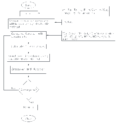
The genetic algorithm code [23] has been adopted for opti- mizing the turbine mean line design with the above formuation. The fitness function is a single objective function defined with different weightages, namely 50% for perfor- mance, 25% for life and 25% for weight of the turbine stage. The effect of change in weightages to (33.3%, 33.3%, 33.3%) are also explored. The fitness function which is formulated as de- scribed above is optimized with constraints on the design var- iables. The initial population size is chosen as 100 generations. The selection function is based on stochastic method. The elite count in reproduction is 2, and the crossover fraction is 0.8 and mutation fraction is 0.01. For convergence of the code, the function tolerance is taken as 1e-06. 0. The three independent design variables for the fitness function, namely Stage Load- ing / Mean radius, Flow coefficient and exit swirl angle with lower and upper bounds for each are defined in the code.
The variable / input vector is given by
Fig. 5. Flow Chart of the Optimization process

The fitness function is defined by
Where K1, K2 and K3 are weight functions.
(1)

(2)
A parametric study has been carried out to study the ef- fect of the design variables independently on efficiency, creep life and weight of the turbine stage. Optimized values of tur- bine efficiency, life and weight with respect to stage loading and flow coefficient and exit swirl angle are obtained for dif- ferent combinations of the weight functions and imposed on the results obtained from the parametric study. The conver- gence plot of the optimization code showing the best fitness and mean fitness values are shown in Figure 6.
The constraints are: α2, β2, β3, M2, M2rel, M3rel, Reaction, flare angles, s/c of the blade and vane, AN2, tip speed, blade metal temperature. In the mean line design, the station 1 referes to the stator inlet, station 2 refers to the rotor inlet and station 3 refers to the rotor outlet. The flow chart for the opti- mization is shown in Fig. 5.

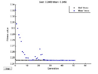
Fig. 6. Converegence Plot of the Opmitization tool

http://www.ijser.org

International Journal of Scientific & Engineering Research Volume 6, Issue 1, January-2015

646

Figure 7 shows the optimized turbine efficiency superim- posed on the parametric study results with respect to flow coefficient for different stage loadings at an optimal swirl an- gle. Similarly Figure 8 and 9 optimized turbine life and weight superimposed on the parametric study results with respect to flow coefficient for different stage loadings and swirl angle respectively. From the figures it can be observed that the op- timum values represent an optimized or compromised solu- tions based on the trends obtained from the parametric study of the mean-line parameters. The optimized value of the flow coefficient and stage loading are 0.84 and 1.55 respectively at an exit swirl angle of 12 degrees, which is the upper bound considering the downstream component performance.

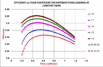
Fig. 7. Efficiency v/s Flow coefficient for differet stage load- ings at constant swirl

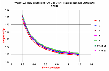
Fig. 8. Wieght v/s Flow Coeffciceint for different stage load- ings

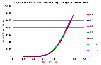
Fig. 9. Life v/s Flow Coefficient for different stage loadings
The optimized flow path and the mean velocity triangles obtained from the optimization of the mean line design are shown in figures 10 & 11

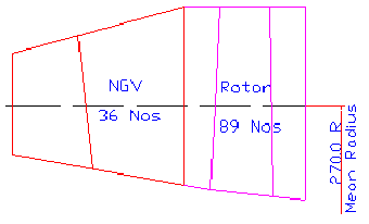
Fig. 10. Optimized Turbine flow path

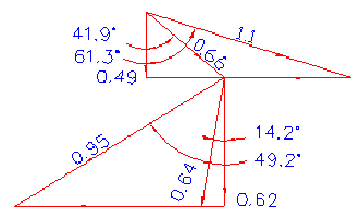
Fig. 11. Optimized Mean Velocity Triangle

The optimization of the mean-line design of a typical low pressure turbine of military aero-gas turbine engine is at-

http://www.ijser.org

International Journal of Scientific & Engineering Research Volume 6, Issue 1, January-2015

647

tempted by using genetic algorithm. The fitness function is formulated by considering the aerodynamic performance, weight and life of the turbine module. The optimized values for different weightages of performance, weight and life are presented in the paper.

The authors wish to thank Shri David John, Scientist for help in preparing the manuscript.

[1] Rolf Dornberger, Dirk Buche and Peter Stoll, “Multidisciplinary Optimization in turbo machinery Design”, European Congress on Computational Methods in Applied Sciences and Engineering, ECCOMAS 2000

[2] George S. Dullikravich, Thomas J. Martin and Zhen-Xue Han, “ Aero- Thermal Optimization of Internally Cooled Turbine Blades”, Minisymposium on Multidisciplinary design, Fourth ECCOMAS Computational Fluid Dy- namics Conference, 1998

[3] K V J Rao, S Kolla, Ch Penchalayya, M Ananda Rao and J Srinivas, “Opti-

mum stage design in axial-flow gas turbines”, Proceedings of the Institution of Mechanical Engineers, Part A: Journal of Power and Energy 2002 216: 433

[4] T.Verstraete and R.A. Van den Braembussche, “Multidisciplinary Optimiza- tion of Turbomachinery components including heat transfer and stress pre- dictions”, Lecture Series 2008-07, Von Karman Institute of Fluid Dynamics

[5] Akira Oyama, Meng-Sing Liou and Shigery Obayashi, “Transonic Axial-flow

Blade Shape Optimization using Evolutionary Algorithm and Three Dimen- sional Navier-Stokes Solver”, AIAA 2002-5642

[6] S. V. Ramana Murthy and S. Kishore Kumar; “Parametric Study Of Axial

Flow Turbine For Mean-Line Design And Blade Element”, GTIndia2012-9589. [7] Carlos M.Fonseca and Peter J.Fleming, “Genetic Algorithms for Mul- ti-objective Optimization: Formulation, Discussion and Generaliza- tion”, Proceedings of Fifth International Conference, San Mateo, CA,

July 1993

[8] Goldberg, D.E., “Genetic Algorithms in Search, Optimization and

Machine Learning”, Addison-Wesley, Reading, Massachusetts, 1989 [9] MATLAB optimtool; “User Documentation,” Version R2010b,The

MathWorks, Inc.J. Williams, “Narrow-Band Analyzer,” PhD disserta-

tion, Dept. of Electrical Eng., Harvard Univ., Cambridge, Mass., 1993. (Thesis or dissertation)

[10] Kacker, S.C.; and Okapuu, U.; “A Mean Line Prediction method for

Axial Flow Turbine Efficiency, “ASME paper 81-GT-58, 1981.

[11] Craig, H.R.M., Cox, H.J.A., “Performance Estimation of Axial Flow

Turbines”, Proceedings of Institution of Mechanical Engineers, 1970-

71.

[12] Taylor,M., “Aero-engine Design: A state of the art”, von Karman

Institute for Fluid Dynamics, April 2003, Lecture series 2003 – 06

[13] Ainley, D.G.; and Mathieson, G.C.R.; “A method of performance

Estimation for Axial Flow Turbines,” British ARC, R & M 2974, 1951.

[14] Glassman J, “Turbine Design and Application”, Volume One and Two,

NASA SP-290, 1973.

[15] Horlock.J.H.; “Axial Flow Turbines,” Butterworths, 1966

[16] Cohen H, Rogers GFC and Saravanamuttoo HIH, “Gas Turbine Theory”,

4th edition, Longman Group Limited, 1996.

[17] Dixon, S.L, “Fluid Mechanics, Thermodynamics of Turbomachinery”,

Pergamon, 1975.

[18] Budugur Lakshminarayana, “Fluid Dynamics and Heat Transfer of

Turbomachinery”, John Wiley & Sons, 1996

[19] K.Harris, G.L.Erickson, R.E.Schwer, “Development of a High Creep Strength, High Ductility, Cast Superalloy for Integral Turbine Wheels – CM MAR-M-247 LC”, 1982 AIME Annual Meeting, Dallas, Texas, Feb 1982

[20] Dodd,A.G., “ Mechanical Design of Gas Turbine Blading in cast Superal-

loys”, Materials Science and Techology, Volume 2, May 1986

[21] R.J.Pera, E. Onat, G.W. Klees, E. Tjonneland: “ A Method to Estimate Weight and Dimensions of Aircraft Gas Turbine Engines”, Volume – I: Method of Analysis, NASA-CR-135170, May 1977

[22] Thomas G. Cunningham Jr., Matthew H.Sandefur, “Integrated Conceptual

design software for Gas Turbine Engines”, ISABE-2009-04

[23] Kishore Kumar S and Wake GC, Optimization Methods and Assessment of

Genetic Algorithm, MUNZ,1990

http://www.ijser.org