optimal number of clusters.
If the distance of significant number of nodes is more than
International Journal of Scientific & Engineering Research, Volume 4, Issue 8, August-2013 1706
ISSN 2229-5518
Optimal Number of Clusters in Wireless Sensor
Networks with Mobile Sink
C.P. Gupta and Dr. Arun Kumar
Abstract-W ireless Sensor Networks (W SNs) employ tiny sensor nodes to observe field and send data from the field to a Base Station. The base station is generally at a fixed location away from the observed field. However, such networks have limited life due to draining of batteries of nodes near the base station quickly in comparison to the nodes away from the base station. Further, data from nodes in close proximity have very little or no variation. Sending data from all the nodes to base station will require larger energy due to longer distances or multiple hops. Clustering has
been found to be an effective solution for such networks. However, efforts to find optimal number of clusters are limited to W SNs with static sink. In this paper, we present an analysis of optimal number of cluster in such networks. The theoretical analysis is supported by simulation results.
—————————— ——————————
In recent years, sensor networks have been deployed for a variety of applications. In few cases viz. fire safety in high rise buildings, the sensors are connected through wires. However, wired networks are rare and do not find large applications. In most cases, the deployment prescribes for a wireless environment. As a consequence, the sensor networks use wireless communication to send the collected data and are thus termed as Wireless Sensor Networks (WSN). Formally, a wireless sensor network (WSN) in its simplest form can be defined as a network of (possibly low- size and low-complex) devices denoted as nodes that can sense the environment and communicate the information gathered from the monitored field through wireless links; the data is forwarded, possibly via multiple hops relaying, to a sink that can use it locally, or is connected to other networks (e.g., the Internet) through a gateway [1].
As presented by Akyildiz [3], the total radio power consumption P c is:
Pc = NT (P T (Ton +T st ) + Pout (Ton )) + NR [P R (Ron +Rst )]
where, PT/R is power consumed by the transmitter/receiver; Pout , the output power of the transmitter; Ton /Ron , the transmitter/receiver on time; Tst /Rst , the transmitter/receiver start-up time and NT/R , the number of times transmitter/receiver is switched on per unit time, which depends on the task and medium access control (MAC) scheme used.
Designing routing protocols for WSNs is challenging due to resource constraints [1, 2]. Research on WSNs has found that clustering the nodes in WSNs reduces the energy consumption significantly as the member nodes transmit
————————————————
• Dr. Arun Kumar is working as Lecturer in Mathematics at Govt. College,
Kota, INDIA. He has authored several papers in the area of mathematical modeling of biological systems. E-mail: arunkr71@gmail.com.
data only to a node within the cluster. The node receiving
data from all the members within the cluster is termed as
Cluster Head (CH). As the CH is within the cluster,
attenuation is only of the order of square of distance as compared to higher power over longer distances. In such networks, CH performs data aggregation on the received data exploiting temporal and spatial proximity thus reducing the total data to be transmitted to the BS. Reduction in distance and amount of data to be transmitted increases network lifetime considerably.
Fixed location of base station or a single base station causes the nodes close to BS die out quicker than rest of the nodes. The phenomenon known as “energy hole problem [3]” makes the network unusable in spite of majority of nodes being still live. Replacing batteries of dead nodes or energy scavenging is generally not possible in WSNs. It suggests that life of network can be prolonged by making the BS mobile. Mobile base station then can travel closer to the node to collect the data from the nodes resulting in energy savings and also avoiding creation of energy holes.
In this paper we present, analysis of optimal number of clusters in networks with mobile base station. In our model, the BS travels very close to the CH. This results in zero attenuation during data collection from CH by the BS. The theoretical results were verified using cluster evaluation techniques. Silhouette Coefficient, Cophenetic Correlation Coefficient, and Spearman Correlation Rank were computed to evaluate the formed clusters. Results establish the theoretical analysis.
Related work is presented in section 2. Mathematical formulation is presented in the next section. Results are presented in section 4. Paper is concluded in section 5.
Clustering in WSNs was first proposed under the protocol LEACH [4]. In LEACH, number of clusters to be formed is determined a priori by assigning a predetermined value of probability of becoming a CH. Rumor [5], TEEN[6], PEGASIS [7] are other well known clustering algorithms.
IJSER © 2013 http://www.ijser.org
International Journal of Scientific & Engineering Research, Volume 4, Issue 8, August-2013 1707
ISSN 2229-5518
However, none of these deliberated upon finding the
optimal number of clusters.
If the distance of significant number of nodes is more than![]()
ε
Bandyopadhyay et al. [8] investigated the optimal number of clusters in hierarchical WSNs. For a network with n nodes deployed as per a homogeneous spatial Poisson process of intensity λ in a square area of side 2a, using
multihop transmission between CH and member nodes;
do =
Kopt =
fs

ε mp
Ns
2π
then,
ε fs M
ε d 2
optimal probability of becoming a CH is![]()
1 3 2
mp toBS
However, none of the above works consider the BS to be
mobile.
![]()
+ +
![]()
![]()
3c (
2 2 )1/ 3
3c 2 + 27c
+3 3c
(27c
+ 4)
p =
Energy available with the node is consumed in![]()
( 2 2
![]()
)1/ 3
3c
2 + 27c
+3 3c
3c
(27c
+ 4) 1
![]()
.
3 2
(i) Data Transmission from Cluster Members (CM) to their respective Cluster Head
![]()
where, c = 3.06a λ .
Ranjan et al. [9] computed the optimal number of clusters in random and grid networks considering single hop and multi hop communication between CH and BS.
FCA [10] uses residual energy parameter with distance to the base station metric of the sensor node to calculate competition radius. In every clustering round, each sensor node generates a random number between 0 and 1. If the random number for a particular node is smaller than the predefined threshold T which is the percentage of the desired tentative cluster-heads, then that sensor node becomes a tentative cluster head. The competition radius of each tentative cluster-head changes dynamically. FCA decreases the competition radius of each tentative cluster- head as the sensor node battery level decreases.
FCM [11] computes the optimal number of cluster heads. Xie and Beni’s (XB) index was used to validate the partitioning. The total energy consumption in transmitting L bits by Ns number of sensors over a distance of dtoCH by the sensor to cluster head and then to the sink at distance
dtoBS having a free space loss coefficient ε is
(ii) Data Reception at Cluster Heads
(iii) Data Aggregation at Cluster Heads
(iv) Data Transmission between Cluster Heads and Base
Station
(v) Computation of Total Energy Consumption
Assumptions:
• Each cluster member sends a data packet of constant length of L bits.
• The cluster head aggregates the data received from all the members with its own data into a frame of L bits.
• The control frames are small in comparison to data frames. Thus, energy consumed in transmitting control frames is negligible in comparison to energy consumed in transmitting data frames and hence, neglected.
Let
k= number of clusters
mi = number of nodes in the ith cluster n= Total number of nodes
E = L(2 Ns E
+ Ns E + ε
(kd 2
+ N d 2 )
Tot
elect
DA fs
toBS
s toCH .
di→CH = Distance between ith node and its cluster head.
The optimal number of clusters Kopt is
Eele c= Energy Consumed in transmitting/ Receiving one bit
Kopt =
Ns 2
![]()
2π 0.765 ,
depends upon coding and modulation
εfs = Free Space Loss Coefficient
and average distance to the base station![]()
d = 0.765 M
Efusion =Energy consumed in data aggregation and computation per bit.
n
toBS 2
![]()
Average Number of nodes in each Cluster=
k
(M = side of deployment area).
3.1.1 Energy consumed in transmission
All the cluster members communicate directly with their respective cluster heads. Further, this communication takes
IJSER © 2013 http://www.ijser.org
International Journal of Scientific & Engineering Research, Volume 4, Issue 8, August-2013 1708
ISSN 2229-5518
place only in the assigned time slot and thus no collision occurs. Hence, energy consumed in each cluster,
Thus, total energy consumed in each round
m−1
Tx ∑
elect fs i→CH
ETotal
=
= ETx−Total + ERx −Total + Ecom
E =
i =1
(L * E
+ L * ε d 2 )
(1)
k m j −1
In the proposed protocol, the base station being mobile,
(n * L * Eelec ) + ∑ ∑
( L * ε
fs * di →CH )
visits the cluster heads to collect the aggregated data.
Because of this, Energy is consumed only in transmitting L
k mij −1
j =1
i =1
(6)
bits of information by k CHs to the base station. No energy
+∑ ∑ L * Eelec + (E fusion * L * n)
loss happens and thus, energy consumption due to this is
j =1
i =1
not considered. Hence, energy consumed in transmitting L
bits by k cluster heads is given by
3.2 Optimal Number of Clusters
ETx−CH
k
= ∑ L * Eelec
j =1
(2)
Let the area observed field is A and the cluster forms a circle with cluster head as center, area of each cluster can be approximated to A/k, one may argue that each cluster can
Total energy consumed in k clusters
be approximated by a circle of radius
A
![]()
, where the
k m j −1 π k
∑ ∑
j=1 i=1
( L*Eelect + L*εfs*d 2
cluster head resides at the center.
opt
ETx−Total = k
+ ∑ L*Eelec
(3)
Since the expected squared distance between a random
j=1
k m j −1
2
![]()
point in a circle of radius S and its center is
2
, the value of
= (n * L * Eelec ) + ∑ ∑
( L*εfs*d 2 ) 2
j=1
i=1
i→CH
di→CH
can be determined with respect to A and k. This
3.1.2 Energy Consumed in Receiving at k cluster heads
Each cluster head receives data from all the cluster members. Thus, ith cluster with mi number of members receives data from mi -1 members. The energy consumed in
can be obtained straightforwardly by drawing a
hypothetical circle around the center (cluster head) and
equating the area of this circle to half of the area of the
original circle (area of the cluster). Solving the resulting equation for squared radius of the hypothetical circle,
receiving at each CH is
mi −1
which is in fact equal to d 2
, yields:
ERx = ∑ LxEelec
i =1
2
i→CH
![]()
= A
2π k
(7)
Thus, the total energy consumed in receiving at k cluster heads
k mij −1
Further, assuming that energy required in fusing one bit is equal to the energy required for transmission/receiving one bit i.e.
ERx−Total = ∑∑ L * Eelec
j =1 i =1
(4)
Efusion = Eelec (8)
Simplifying equation (6) and substituting the equation (7)
3.1.3 Energy Consumed in data aggregation and computation at the cluster head
and (8) in (6), we get
k A
The CH aggregates data from all the members and also its own data. Thus the total energy consumed in aggregating
at k cluster heads
ETotal = (3n − k )* L * Eelec + ∑ (m j − 1)* L * ε fs *
j =1
(n − k )
![]()
2π k
(9)
Ecom = E fusion * L * n
(5)
= (3n − k ) * L * Eelec +
![]()
2π k
* L * A * ε fs
To minimize the total energy consumption, the optimal![]()
nAε fs
value of clusters works out to kopt = − π E .
2 elec
IJSER © 2013 http://www.ijser.org
International Journal of Scientific & Engineering Research, Volume 4, Issue 8, August-2013 1709
ISSN 2229-5518
The sign of the expression under square root is insignificant and thus is neglected. Hence, optimal number of clusters is obtained as
kopt =
![]()
nAε fs
2π Eelec
(10)
Bandyopadhyay et al. [8] found the number of clusters considering multihop communication within cluster and
also between CH and BS. Anwar et al. [12] considered re- transmission of lost packets during communication between CH and BS. The above results are not suitable for our model due to following reasons:
Our network model assumes single hop communication between CM and CH.
In our network model, the sink is mobile and moves very close to the CH for PULLING the aggregated data from CH. Thus, path loss between CH and sink is insignificant. Further, due to proximity of sink with CH at the time of data collection, probability of error is negligible not requiring retransmission.
Simulations were carried out on a network of 100 nodes deployed in a square area of 100 x 100. 100 samples were generated and the network was clustered using Hierarchical Agglomerative Clustering [13-15]. The network was clustered using for techniques namely Single Linkage, Average Linkage, Complete Linkage and Ward’s Linkage. Evaluation is based on computing three parameters namely (i) Silhouette Coefficient (SC) (ii) Cophenetic Correlation Coefficient (CPCC) and (iii) Spearman Correlation Rank (SCR). Results are shown in Fig. 1 to 3.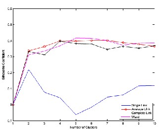
Fig 1: Average Silhouette Coefficient
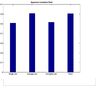
Fig 2: Average Cophenetic Correlation Coefficient
Fig 3: Average Spearman Correlation Rank
Theoretical value for optimal number of clusters as computed works out to be 6. Value of Silhouette Coefficient for average linking is the highest for this number of clusters. As per [13, 14] optimal number of clusters is represented by the highest value of the coefficient. Further, CPCC is used to evaluate the optimal linkage in the given data set. The higher value of coefficient suggests the linkage method for clustering the data. For randomly generated points in our simulation, for all the runs, value was the highest for average linking. The SCR was computed between Euclidean Distance and Cophenetic Distance. Cophenetic Distance is measured as the height of the dendrogaram at which the node was first merged into another cluster. Higher value point well clustering. Our results suggest that for randomly deployed WSNs, average linkage results in optimal clustering.
IJSER © 2013 http://www.ijser.org
International Journal of Scientific & Engineering Research, Volume 4, Issue 8, August-2013 1710
ISSN 2229-5518
References
[1] Gupta, C P, Kumar Arun: "Wireless Sensor Networks: A Review", International Journal of Sensors, Wireless Communications and Control, 2012, Vol. 2, No. 3, Pg
1-12.
[2] Akyildiz, Ian F., et al. "Wireless sensor networks: a survey." Computer networks 38.4 (2002): 393-422.
[3] Ahmed, Nadeem, Salil S. Kanhere, and Sanjay Jha. "The holes problem in wireless sensor networks: a survey." ACM SIGMOBILE mobile Computing and Communications Review 9.2 (2005): 4-18.
[4] Heinzelman, Wendi Rabiner, Anantha Chandrakasan, and Hari Balakrishnan. "Energy-efficient communication protocol for wireless micro-sensor networks." System Sciences, 2000. Proceedings of the
33rd Annual Hawaii International Conference on.
IEEE, 2000.
[5] Braginsky, David, and Deborah Estrin. "Rumor routing algorithm for sensor networks." Proceedings of the 1st ACM international workshop on Wireless sensor networks and applications. ACM, 2002.
[6] Manjeshwar, Arati, and Dharma P. Agrawal. "TEEN: a routing protocol for enhanced efficiency in wireless sensor networks." 1st International Workshop on Parallel and Distributed Computing Issues in Wireless Networks and Mobile Computing. Vol. 22.
2001.
[7] Lindsey, Stephanie, and Cauligi S. Raghavendra. "PEGASIS: Power-efficient gathering in sensor information systems." Aerospace conference proceedings, 2002. IEEE. Vol. 3. IEEE, 2002.
[8] Bandyopadhyay, Seema, and Edward J. Coyle. "An energy efficient hierarchical clustering algorithm for wireless sensor networks." INFOCOM 2003. Twenty- Second Annual Joint Conference of the IEEE Computer and Communications. IEEE Societies. Vol.
3. IEEE, 2003.
[9] Ranjan, Ravi, and Subrat Kar. "A novel approach for finding optimal number of cluster head in wireless sensor network." Communications (NCC), 2011
National Conference on. IEEE, 2011.
[10] Godbole, Vaibhav. "Performance Analysis of Clustering Protocol Using Fuzzy Logic For Wireless Sensor Network." IAES International Journal of Artificial Intelligence (IJ-AI) 1.3 (2012).
[11] Raghuvanshi, Ajay Singh, et al. "Optimal number of clusters in wireless sensor networks: a FCM approach." International Journal of Sensor Networks
12.1 (2012): 16-24.
[12] Sadat, Anwar, and Gour Karmakar. "Optimum Clusters for Reliable and Energy Efficient Wireless Sensor Networks." Network Computing and Applications (NCA), 2011 10th IEEE International Symposium on. IEEE, 2011.
[13] Tan, Pang-Ning, “Introduction to data mining”.
Chapter 8, Pearson Education India, 2007.
[14] Tryfos, Peter,” Methods for Business Analysis and Forecasting: Text and Case”, Chapter 15, John Wiley, ISBN: 0-471-12384-6, 1998.
IJSER © 2013 http://www.ijser.org