International Journal of Scientific & Engineering Research, Volume 6, Issue 4, April-2015 148

ISSN 2229-5518

On The Behavior of Strategies in Iterated

Games Between Relatives

Essam EL-Seidy ,Salah El Din S.Hussien and Ali M. Almuntaser

Abstract — The theory of iterated games provide a system framework to explore the players' relationship in a long-term. In this paper we consider the iterated prisoner's dilemma game (IPD) played between relatives . Two state automata are used to play infinitely iterated the two players where each action can be mis-implemented with small error probability. the payoff matrix using the perturbation approach is computed . Using a different values of the average relatedness between players and different values of the payoff variables (R; S; T; P) , the behavior of strategies for iterated prisoner's dilemma game in each situation is studied .

Keywords : Repeated Games, Transition matrix, Finite automata, Perturbed Payoff.

——————————  ——————————

1 INTRODUCTION

Game theory provides a quantitative framework for analyzing the behavior of rational players . The theory of iterated games in particular provide a system framework to explore the players' relationship in a long-term. It has been an important tool in the behavioral and biological sciences and it has been often invoked by economists, political scientists, anthropologists and other scientists who were interested in human cooperation (Axelrod 1984, Aumann 1981,Fudenberg and Mask 2007; 1990).
The prisoner's dilemma game (Rapoport and Chammah
1995) is the most famous example of iterated games . The (IPD) is now regarded as an ideal experimental platform for the evolution of cooperation among selfish players and it attracts wide interest since Robert Axelrod's IPD tournaments . However, the publication of Axelrod's book in the 1980s was largely responsible for bring this research to the attention of other areas outside of game theory, including evolutionary computation, conflict resolution, evolutionary biology, networked computer systems and promoting cooperation between opposing countries. Despite the large literature base that now exists this is an outstanding area of research.
In this paper, we study the iterated prisoner's dilemma game in which there is a relationship between the players . The average relatedness between the players is given by r,

————————————————

 Author name is currently pursuing masters degree program in electric power engineering in University, Country, PH-01123456789. E-mail: author_name@mail.com

 Co-Author name is currently pursuing masters degree program in electric

power engineering in University, Country, PH-01123456789. E-mail:

author_name@mail.com

(This information is optional; change it according to your need.)

which is a number between 0 and 1. A simple way to study games between relatives was proposed by Maynard Smith for the Hawk-Dove game ( Hines and Smith 1979 ; Grafen 1979 ).
In iterated prisoner's dilemma, the two players have two
options, either to Cooperate (C) or to defect (D). In one-shot prisoner's dilemma game ,the strategy D is the best, and it dominates the cooperative option . But if this game played repeatedly many times then the picture will change. In this situation the strategy D will not be the dominant strategy for a long time. In iterated games, the number of possible grows exponentially with the number of rounds in the game (Nowak at el .1995 ; Rubinstein 1986 ).
We assume that ,when the players plays the iterated
Prisoner's Dilemma there is some noise , i.e. In each round, a player makes a mistake with probability _ leading to the opposite move. Since there is a lot of strategies of (IPD) , we just consider all strategies that can be implemented by deterministic _nite state automata with one or two states. Finite state automata have been used extensively to study the iterated games . In our case, we have two states each state is labeled by C or D.
In state C the player will cooperate in the next move ; in state D the player will defect. Each strategy starts in one of those two states. Each state has two outgoing transitions (either to the same or to the other state): one transition specifies what happens if the opponent has cooperated and one if the opponent has defected (Zagorsky at el.2013 ; Nowak at el.1995 ) .
In (Nowak at el. 1995 ) they studied prisoner's dilemma where they used the played repeatedly by two-state automata

IJSER © 2015 http://www.ijser.org

International Journal of Scientific & Engineering Research, Volume 6, Issue 4, April-2015 149

ISSN 2229-5518

, they computed the 16_16 payoff matrix for limiting case of vanishingly a small noise term affecting the interaction . In this paper we define the transition rule of each automaton that depends on the initial state of the game and on the payoff of last move , and we compute the payoff matrix of iterated prisoner's dilemma games in which there is a relationship between the players . Then we describe the method that we shall follow to compute the 16 x16 payoff matrix for iterated prisoner's dilemma game with noise played by finite state automata. After calculating the payoff matrix we study the effect of different values of average relatedness and different values for the payoff values (R; S; T; P) on the behavior of the
16 strategies .

2 Prisoner's Dilemma Between Relatives

The Prisoner's Dilemma (PD) is a non-zero sum game formulated by the mathematician Tucker building on the ideas of Flood and Dresher in 1950 . Since then, it has been discussed extensively by game theorists, economists, mathematicians, political scientists, biologists, philosophers, ethicists, sociologists, and the computer scientists ( Brunauer at el 2007). Many variations of the Prisoner's Dilemma have been devised, one of them being the Iterated Prisoner's Dilemma (IPD), which is at the center of attention in this paper. In this game , the two players have two options, either to Cooperate (C) or to defect (D) and the payoff values

are traditionally called T (for temptation to betray a

betrayed by him or her (S) . We can represent this game by the following payoff matrix :

C D

C ( ) (1)

D

Now , we assume that this game is played between relatives. A simple way to study games between relatives was proposed by Maynard Smith for the Hawk- Dove game (Hines and Smith 1979 ; Grafen 1979 ). Consider a population where the average relatedness between players is given by r, which is a number between 0 and 1.There are two possible methods to study the games between relatives. The "inclusive fitness " method adds to the payoff of a player r times the payoff to his co- player .The personal fitness method, proposed by Grafen 1979 modifies the fitness of the player by allowing for the fact that a player is more likely than other players of the population to meet co- player adopting the same strategy as himself. We regard the inclusive fitness method to study the iterated prisoner's dilemma that played by finite state automata and subjected to a small error (Hines and Smith 1979 ). If we assume that there is a relationship between the players , then by using the inclusive fitness method , the payoff matrix of the prisoners dilemma game is given by

cooperating opponent), S (for sucker's payoff when being betrayed while cooperating oneself), P (for

C

C ( )

D (

D

( )) (2)

punishment when both players betray each other), and R (for reward when both players cooperate with each other). Their values vary from formulation to formulation of the prisoner's dilemma. Nevertheless, the inequalities S < P < R < T and 2R > T +S are always observed between them. The last one ensures that cooperating twice (2R) pays more than alternating one's own betrayal of one's partner (T) with allowing oneself to be

where r is the average relatedness between players ,

which is a number between 0 and 1.

3 Finite Automata and Transition Rule

The potential of the automata theory for the analysis of games was first suggested in the economics literature by Aumann (1981). Finite-state automata have been used extensively to study iterated games including prisoner's dilemma (Zagorsky at al. 2013 ) . In this paper we use an

automata with two states as we mentioned that in

IJSER © 2015 http://www.ijser.org

International Journal of Scientific & Engineering Research, Volume 6, Issue 4, April-2015 150

ISSN 2229-5518

introduction , each state of the automaton is labeled by C or D , in the state C the player will cooperated in the next move , in the state D the player will defect .All the strategy starts in one of those two states . Each state has two outgoing transition : one transition specifies what happens if the opponent has cooperated and one if the opponent defected.

There are 32 automates with two different states,

but some of these automaton describe automata with the same behavior . Thus there are only 26 automata encoding unique strategies (Nowak at el.

1995 ; El Seidy at el. 2013) . These strategies include AllC , AllD , Tit-For-Tat (TFT) and Win-Stay, Lose- shift (WSLS)(Fig.1).

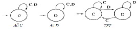
Fig.1

Each round leads to one of the four possible outcomes (C,C) , (C,D) , (D,C) or (D,D), where the first position denotes the option chosen by the player and the second that of the co-player. These outcomes , from the player's point of view, are specified by his payoff R , S , T or P, which can be numbered by 1 , 2 , 3 , 4. The 16 possible transition rules can be defined by a quadruple (p1 , p2 , p3 , p4) of zeros and ones .Where pi denotes the probability to cooperated after each of the four outcomes (C,C),(C,D),(D,C) and (D,D). Thus (1, 1, 1, 1) is the rule of cooperate (AllC) and (0, 0, 0, 0) is the rule of defect (AllD), while (1, 0, 1, 0) is the rule of imitating the adversary's last move. The automata using this rule and with initial state C plays Tit-for- Tat. TFT starts in state C and subsequently does

whatever the opponent did in the last round . This

only recover from a single error by another error (Zagorsky at el. 2013 ) . To simplify , we label these rules by Si where i ranges from 1 to 15 and is the integer given . Hence S0 is AllD and S10 is Tit-for- Tat.

4 The Competitions Between Strategies with

Noise

How one rule matches against another depends on the initial condition of this rule. For example , consider the automaton with rule S12 = (1, 1, 0, 0) against the automaton with rule S14 = (1, 1, 1, 0) , therefore :
(a) If both automaton start with C, they keep playing C
forever, The sequence is: S12 : C C C C C C C C::::: S14 : C C C C C C C C:::::
(b) If both automaton start with D , they keep playing D
forever ,we get:
S12 : D D D D D D D:::: S14 : D D D D D D D::::
(c) If S12 starts with C and S14 with D , we get: S12 : C C C C C C C::::
S14 : D D C C C C C::::
(d) If S12 start with D and S14 with C, the result is: S12 : D D D D D D D::::
S14 : C C C C C C C:::::
In the infinitely iterated game , the payoff is the average payoff per round , in our example, the player who use the transition rule S12 get the payoff R(1 + r) in cases (a) and (c), and P(1 + r) in case (b), and T + rS in case (d).
Now, if we assume that the implementation of a move is
subject to error. This means that there is a small probability ε >
0, that one state is replaced by another. The corresponding transition rule in this case is given by a quadruple like Si but with ε instead of 0 and 1- ε instead of 1. The problem now is to compute the payoff for strategy Si (ε) against Sj (ε).For more generally, let us consider a strategy E = (e1 , e2 , e3 , e4) and F = (f1 , f2 , f3 , f4) where ek and fk are the probability to play C after outcome k ( k = 1, 2, 3, 4 ) . Therefore , we get the transition matrix between the four states R, S, T and P as shown in the stochastic matrix (3).

strategy is very successful in an error-free M=

environment , but in a noisy environment TFT

(3)

achieves a very low payoff against itself since it can

(We note the interchange of 2 and 3, due to the fact that one
player's S is the other player's T ). If the matrix M is irreducible

IJSER © 2015 http://www.ijser.org

International Journal of Scientific & Engineering Research, Volume 6, Issue 4, April-2015 151

ISSN 2229-5518

(as is always the case when 0 < ek , fk < 1 for all k , and for particular if E and F correspond to strategies Si ), the matrix
M has a unique left eigenvector α = (α1 , α2 , α3 , α4)to the eigenvalue 1 such that 0 < αk for k = 1, 2, 3, 4 and k = 1 . These
∑ αk denote the relative frequencies of the states k of the corresponding Markov chain. They specify the limit in the mean payoff for strategy E against strategy F which is α1R + α2S + α3T + α4P ,Since our game is played between relatives as we assumed , therefore the payoff will be α1R(1+r)+ α2(S+rT)+ α3(T +rS)+ α4P(1+r) .the F player's payoff is obtained by interchanging α2and α3 .
Now , for any noise level ε > 0, we can compute the payoff obtained by the automaton using transition rule Si against the automaton using transition rule Sj using the following approach : (we will exemplify it for S12 against S14 ). The
four possible initial condition leads to three possible stationary
states R1;R2, and R3 ,where R1 denotes the run where the both player use C. while R2 is the run where the S12-player plays D and S14-player plays C and R3 is the run where the both player use D. Now , suppose we are in regime R1. A rare perturbation cause S12-player to play D, this leads to regime R2 with probability 1/2 . Suppose that the perturbation happened in regime R2. With probability 1/2 , it cases the S12- player to switch from D to C .If this happens while S14-player plays C, we are in regime R1, but if S14-player plays D, this leads to regime R3. Suppose now that the perturbation occurs in regime R3 , with probability 1/2 , it cases the S12-player
to switch from D to C if this happens while S14-player plays
D, we are in regime R1 suppose now that the perturbation a_ects the S14-player, He plays C instead of D, while S12- player plays D, this leads to regime R2.Thus the perturbation of R1 leads with probability 1/2 to R2 , and the perturbation of R2 leads with probability 1/2 to R1 and with probability 1/2 to R3 , while R3 leads with probability 1/2 to R1 and with probability 1/2 to R2. The corresponding transition matrix is:




(4)


( )
and the corresponding stationary distribution is ( 1/2 ; 1/3 ;
1/6).Therefore ,the S12-player receives the average payo_ 1
/2R(1 + r) + 1/3 (T + rS) + 1/6P(1 + r) per round. This method , repeated for each of the 256 entries, leads to the 16 _ 16 payo_ matrix (Table 2).Now, we said that a strategy Si is out competed by strategy Sj if the following conditions are
satis_ed : V (Sj ; Si) _ V (Si; Si)and V (Sj ; Sj) _ V (Si; Sj).For
example, the payo_ matrix between the S12-player and S14- player ,after substituting with Axelrod's payo_ values (R = 3; S
= 0; T = 5; P = 1) and assume that the average relatedness between the players is 0:5 , is given by :

𝑓8 ( ) (5)

𝑓9

Then , we notice that V (S14; S14) > V (S12; S14) , but V (S14;
S12) _ V (S12; S12) , therefore the strategy S12 is not out competed by the strategy S14 .

5 The E_ciency of Average Relatedness on the

Behavior of Strategies

In this section we study the behavior of strategies and the e_ect of the average relatedness (r) between players on cooperative , defective and other behaviors in competition between strategies . we use di_erent values for r and di_erent values for the variables of payo_ values (R; S; T; P).In Table 1 we summarize all strategies that out compete the strategy Si in each situation that we studied and we see that :

(a)For the payo_ values (R = 3; S = 0; T = 5; P = 1) and

for r = 0:0001 and r = 0:999 , we get from tables (1); (3) and (4) : If the average relatedness between players was small, such that r = 0:0001 , then we see that all strategies are out competed by at least two other strategies . also we note that the strategy S0 (AllD)

can defeat the greatest number of strategies (exactly

12), while the strategy S6 (idiot strategy) cannot defeat any other strategy . Strategies S14 and S15 are the weakest strategies , they out competed by exactly

11 strategies . here , the cooperative strategies are

invaded by a defective strategies. In this case we note that the strategy S9 (called Win-Stay Lose-Shift or Pavlov) is out competed by three strategies , which mean whenever the average of relatedness is low , then the strategy S9 (and the other cooperative strategies) is invaded by other strategies. The strategy TFT or S10 make a good work and defeat the defective strategies like Grim (S8) , AllD( S0) ,and S1 . If the average relatedness between players was large , such that r = 0:999 , then we see that all strategies

IJSER © 2015 http://www.ijser.org

International Journal of Scientific & Engineering Research, Volume 6, Issue 4, April-2015 152

ISSN 2229-5518

except S9; S14 and S15 are out competed by at least three other strategies .the strategies S9; S14 and S15 are defeat all other strategies while the strategy S6 cannot defeat any other strategy . Also when the average relatedness between players is high then the strategies S0 = (0; 0; 0; 0) (a defective strategy) and S8

= (1; 0; 0; 0)(a retaliator who never relents after a

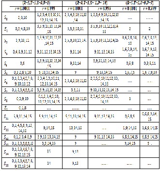
defection ) are out competed by the largest number of strategies (exactly by 11 strategies). The ordered paired of equilibrium strategies in both cases are (S0; S8); (S3; S12); (S5; S10) and (S14; S15).

Table 1: the strategies that out compete the strategy Si (i = 0; 1;
; 15) with di_erent values of R; S; T; P and r.
(b) If the payo_ values were as follow (R = 0; S = �1; T = 1; P =
�10) (called the chicken game) and for r = 0:0001 and 0:999, from tables (1); (5) and (6) : for r = 0:0001 , the defective strategies show some activity and trying to avoid invasion
by other strategies , but they cannot avoid TFT and WSLS
strategies. The strategy WSLS is the strongest strategy and no other strategy can defeat it .Some strategies like S5 are ambitious and try to invade other strategies . The ordered paired of equilibrium strategies are (S0; S8); (S3; S12); (S5; S10); (S9; S11); (S11; S13); (S11; S14); (S11; S15)and(S14; S15).If we assume that r = 0:999 the cooperative strategies S13; S14; S15 and the WSLS(S9) or Pavlov strategy are dominating other strategies and no other strategy can defeat any one of them . In
this case the defective strategies as GRIM (S8) and AllD are invaded by cooperative strategies and then the cooperative behavior will be evolve between the players.The ordered paired of equilibrium strategies are (S0; S8); (S3; S12); (S5; S10); (S9; S11); (S9; S13); (S9; S14); (S9; S15); (S11; S13); (S11; S14); (S11; S15); (S13; S14); (S13; S15); and (S14; S15).
(c) In which the payo_ values were (R = 5; S = 0; T = 1; P = 3)
and r = (0:0001and 0:999), therefore from tables (1); (7) and (8) we see that when the average relatedness between players is small , such that r = 0:0001,we see that there is a strong competition between defective and cooperative strategies. some strategies such as WSLS , AllC and AllD, no other strategy can out compete them, however if the average relatedness between players was large , such that r = 0:999, the defective strategies like Grim(S8) become stronger and no other strategy can defeat it . Some strategies are not a_ected by the values of r such as WSLS or Pavlov, AllC and AllD and other strategies .In two cases the ordered paired of equilibrium strategies are (S0; S8); (S3; S12); (S5; S10) , and (S14; S15).

Conclusion

We have studied in this paper the iterated games played by
_nite state automata . We consider a relationship between the players who plays this game, this relationship is given by an average relatedness parameters r where 0 _ r _ 1. We assumed that the automata are subjected to some small error , this error due to implementation of what the other player does .We computed the 16_16- payo_ matrix of iterated prisoner's dilemma game between relatives with noise which played
by _nite state automata . We studied this game with di_erent
values of R; S; T and P and di_erent values of average relatedness between players .
For the payo_ values (R = 3; S = 0; T = 5; P = 1) and for r = 0:999
and r = 0:0001 we concluded that , all strategies are out competed by at least two other strategies except for , the strategy WSLS(S9)or Pavlov if r=0.999 there is no strategy can defeat this strategy . Also the strategy S6 does not a_ected by the relatedness average , it is a weak strategy in both cases. We saw that whenever there is a large degree of kinship , the cooperation evolve between the players, and the cooperative strategies are dominate . while if there is a small degree of kinship , the defective strategies will dominate and the defective behavior between players will evolve. If we change the order of payo_ values such that(R = 0; S = �1; T = 1; P = �10) (for the chicken game) , we found that whenever a small
degree of kinship between players , the defective strategies

IJSER © 2015 http://www.ijser.org

International Journal of Scientific & Engineering Research, Volume 6, Issue 4, April-2015 153

ISSN 2229-5518

show some activity and trying to avoid invasion by other strategies . In this case the strategy WSLS(S9) or Pavlov is the strongest strategy and doesn't a_ected by the values of r .In case that R > P > T > S and such that (R = 5; S = 0; T = 1; P = 3) , there is a strong competition between defective and cooperative strategies . Almost all the strategies are not signi_cantly a_ected by degree of kinship between the two players . the strategy TFT(S10)for large degree of kinship between players is not successful and exposed to invasion
by AllD ,WSLSor Pavlov , Grim , AllC and other strategies
.here the direct reciprocity behavior in not the best respond for each players .

References

[1] R.J. Aumann,” Survey of repeated games, Essays in game theory and mathematical economics in honor of Oskar Morgenstern”, 4 (1981) 11-42.
[2] A. Grafen, “The hawk-dove game played between
relatives”, Animal Behaviour, 27 (1979) 905-907.
[3] R.M. Axelrod, “The evolution of cooperation”, Basic books,
2006.
[4] D. Abreu and A. Rubinstein,” The structure of Nash equilibrium in repeated games with finite automata”, Econometrical : Journal of the Econometric Society, (1988)
1259-1281.
[5] D. Fundenberg, E. Maskin, Evolution and cooperation in noisy repeated games, The American Economic Review, (1990)
274-279.
[6] D. Fudenberg, and E. Maskin (2007), “Evolution and
Repeated Games,” mimeo.
[7] M.A. Nowak, K. Sigmund and E. El-Sedy,” Automata, repeated games and noise”, Journal of Mathematical Biology,
33 (1995) 703-722.
[8] W.G.S. Hines and J.M. Smith,” Games between relatives”, Journal of Theoretical Biology, 79 (1979) 19-30.
[9] E. El Seidy, H.K. Arafat and M.A. Taha, “The Trembling Hand Approach to Automata in Iterated Games”, Mathematical Theory and Modeling, 3 (2013) 47-65.
[10] J.S. Banks and R.K. Sundaram , “Repeated games, finite
automata, and complexity”, Games and Economic Behavior, 2 (1990) 97-117.
[11] A. Rapoport and A. Chammah,” The Prisoner's
Dilemma”, Univ. of Michigan Press, Ann Arbor (1995),. [12] A. Rubinstein,” Finite automata play the repeated prisoner's dilemma”, Journal of economic theory, 39 (1986) 83-
96.
[13] E. EL-sedy and Z. Kanaya ,” the perturbed payoff matrix of strictly alternating prisoner's dilemma game”, Far East J.Appl.Mat.2(2)(1998),125-146.
[14] B.M. Zagorsky, J.G. Reiter, K. Chatterjee and M.A. Nowak,” Forgiver triumphs in alternating Prisoner's Dilemma”, PloS one, 8 (2013) e80814.

IJSER © 2015 http://www.ijser.org

International Journal of Scientific & Engineering Research, Volume 6, Issue 4, April-2015 154

ISSN 2229-5518

Table 1 . the payoff matrix of repeated prisoner’s dilemma between relatives with error in implementation

( ) ( ) ( )

( ) ( )

( )

( ) ( )

( ) ( )

( )

( ) ( ) ( ) ( )

( ) ( )

( )

( ) ( )

( ) ( )

( )

( ) ( ) ( )

( ) ( )

( ) ( ) ( )

( )

( ) ( )

( ) ( ) ( )

( ) ( ) ( )

( )

( )

8 ( ) ( )

( ) ( )

( ) ( )

9

( ) ( ) ( )

( )

( ) ( ) ( ) ( )

( ) ( )

( ) ( )

( )

( ) ( )

( )

( ) ( )

( ) ( )

(3S+T+P)/6+r*(3T+S+P)/6 ( )

( ) ( )

( ) ( )

( )

( ) ( )

( )

IJSER © 2015 http://www.ijser.org

International Journal of Scientific & Engineering Research, Volume 6, Issue 4, April-2015 155

ISSN 2229-5518

8 9

( ) ( )

( ) ( )

( ) ( ) ( )

( )

( )

( ) ( ) ( ) ( )

( ) ( ) ( )

( ) ( )

( ) ( ) ( ) ( )

( ) ( ) ( ) ( )

( ) ( ) ( )

( )

( )

( ) ( )

8 ( ) ( ) ( )

( ) ( )

9 ( )

( )

( ) ( )

( ) ( )

( )

( ) ( )

( ) ( )

( ) ( ) ( ) ( )

( )

( ) ( ) ( ) ( )

( )

( ) ( ) ( ) ( )

( )

( ) ( ) ( ) ( )

( )

IJSER © 2015 http://www.ijser.org

International Journal of Scientific & Engineering Research, Volume 6, Issue 4, April-2015 156

ISSN 2229-5518

( ) ( ) ( )

( ) ( )

( ) ( ) ( ) ( )

( )

( ) ( ) ( ) ( )

( )

( ) ( ) ( )

( )

( )

( ) ( ) ( ) ( ) ( )

( ) ( ) ( ) ( )

( )

( ) ( ) ( ) ( ) ( )

8

9 ( )

( ) ( ) ( ) ( )

( ) ( ) ( ) ( ) ( )

( )

( ) ( ) ( ) ( )

( ) ( ) ( ) ( ) ( )

( ) ( ) ( ) ( ) ( )

( ) ( )

( )

( ) ( )

( ) ( )

( )

( ) ( )

IJSER © 2015 http://www.ijser.org

International Journal of Scientific & Engineering Research, Volume 6, Issue 4, April-2015 157

ISSN 2229-5518

Table 2 . the payoff matrix of repeated prisoner’s dilemma between relatives with error in implementation with Axelrod values (R=3,T=5,S=0,P=1) and r=0.0001

Table 3 . the payoff matrix of repeated prisoner’s dilemma between relatives with error in implementation with Axelrod values (R=3,T=5,S=0,P=1) and r=0.999

Table 4 . the payoff matrix of repeated prisoner’s dilemma between relatives with error in implementation with Axelrod values (R=0,T=1,S=-1,P=-10) and r=0.0001

IJSER © 2015 http://www.ijser.org

International Journal of Scientific & Engineering Research, Volume 6, Issue 4, April-2015 158

ISSN 2229-5518

Table 5 . the payoff matrix of repeated prisoner’s dilemma between relatives with error in implementation with Axelrod values (R=0,T=1,S=-1,P=-10) and r=0.999

Table 6 . the payoff matrix of repeated prisoner’s dilemma between relatives with error in implementation with Axelrod values (R=5,T=1,S=0,P=3) and r=0.0001

IJSER © 2015 http://www.ijser.org

International Journal of Scientific & Engineering Research, Volume 6, Issue 4, April-2015 159

ISSN 2229-5518

Table 7 . the payoff matrix of repeated prisoner’s dilemma between relatives with error in implementation with Axelrod values (R=5,T=1,S=0,P=3) and r=0.999

IJSER © 2015 http://www.ijser.org

International Journal of Scientific & Engineering Research, Volume 6, Issue 4, April-2015 160

ISSN 2229-5518

, , , ,

9 9

9 9 9

8 9 8 9

9 9 9 9

Table 8: table of strategies that outcompete the strategy (i = 0,1,…,15) with different values of R,S,T and P, and different averages of relatedness between players

IJSER © 2015 http://www.ijser.org