International Journal of Scientific & Engineering Research, Volume 5, Issue 12, December-2014 1250
ISSN 2229-5518
Numerical Solution of Stiff Delay and Singular
Delay Systems using Leapfrog Method
S. Sekar and M. Vijayarakavan
Abstract— In this paper, a new method of analysis of the stiff delay and singular delay systems using Leapfrog method is presented. To illustrate the effectiveness of the Leapfrog method, an example of the stiff delay and singular delay systems has been considered and the solutions were obtained using methods taken from the literature (single-term Haar wavelet series [6]) and Leapfrog method and are compared with the exact solutions of the stiff delay and singular delay systems. Error graphs are presented to highlight the efficiency of the Leapfrog method.
Index Terms— Haar wavelet, Single term Haar wavelet series, Leapfrog method, singular delay systems, stiff delay systems.
—————————— ——————————
system of DDEs is considered stiff when it contains pro- cesses of widely different time scales. From a computa-
tional point of view the stiffness implies that, while solving numerically the corresponding initial value problem by a giv- en method with assigned tolerance, a stepsize is restricted by stability requirements rather than by the accuracy demands. The response of an immune system cannot be represented cor- rectly without the hereditary phenomena being taken into ac- count: cell division, differentiation, etc. The kinetic parameters of the models represent high-rate (molecular) and slowrate (cellular) interactions in the immune system that span a time scale from seconds to days. Therefore, the systems of DDEs
frog method for solving stiff delay and singular delay systems is introduced. In Section 3 presents general form of stiff delay and singular delay systems. In Section 4 and 5, the Leapfrog and STHWS [4-5, 7-9] method for solving stiff delay and sin- gular delay systems is solved. We refer [4-9] for the numerical treatment of stiff delay and singular delay systems.
In mathematics Leapfrog integration is a simple method for numerically integrating differential equations of the form
x = F (x) , or equivalently of the form v = F (x), x ≡ v , particu-
larly in the case of a dynamical system of classical mechanics.
appearing in immune response modelling are typically stiff.
Now day, the phenomena of time delay in many practical
Such problems often take the form
x = −∇V (x) , with energy
systems have had many scholars’ much attention. And many excellent results for the systems with time delay have been obtained [1–18]. Especially for the relationship between eigen- value and stability of differential systems with delay, much
![]()
![]()
function E(x, v) = 1 v 2 + V (x) , where V is the potential energy
2
of the system. The method is known by different names in
different disciplines. In particular, it is similar to the Velocity
Verlet method, which is a variant of Verlet integration. Leap-
achievement has been gotten. But we notice that a lot of prac-
frog integration is equivalent to updating positions
x(t ) and
tical systems, such as economic systems, power systems and
so on, are singular differential systems with delay. In [10–18],
velocities
v(t ) = x(t )
at interleaved time points, staggered in
authors have discussed the singular differential systems, even the singular differential systems with delay, and have gotten some consequences. But up to now, for the relationship be- tween eigenvalue and stability of singular differential systems with delay, there is hardly effective verdict.
In this article introduced a numerical method for ad-
such a way that they 'Leapfrog' over each other. For example,
the position is updated at integer time steps and the velocity is
updated at integer-plus-a-half time steps.
Leapfrog integration is a second order method, in con-
trast to Euler integration, which is only first order, yet requires
the same number of function evaluations per step. Unlike Eu- ler integration, it is stable for oscillatory motion, as long as the
dressing stiff delay and singular delay systems by an applica-
time-step
∆t is constant, and
![]()
∆t ≤ 2 w . In Leapfrog integra-
tion of the Leapfrog method which was studied by S.Sekar
and team of his researchers [4-5, 7-9]. In Section 2, the Leap-
————————————————
• Department of Mathematics, Government Arts College (Autonomous), Cherry road, Salem – 636 007, Tamil Nadu, India
tion, the equations for updating position and velocity are
![]()
xi = xi −1 + vi −1 2∆t,
ai = F (xi )
![]()
![]()
vi +1 2 = vi −1 2 + ai ∆t,
E-mail:sekar_nitt@rediffmail.com
where
![]()
xi is position at step i, vi +1 2 , is the velocity, or first de-
• Department of Mathematics, V.M.K.V. Engineering College, Salem – 636
rivative of x, at step
![]()
i + 1 2, ai = F (xi ) is the acceleration, or
308, Tamil Nadu, India
E-mail:vijayarakavan.m@rediffmail.com
second derivative of x, at step i and ∆t is the size of each time step. These equations can be expressed in a form which gives
IJSER © 2013 http://www.ijser.org
International Journal of Scientific & Engineering Research, Volume 5, Issue 12, December-2014 1251
ISSN 2229-5518
velocity at integer steps as well. However, even in this syn-
for
0 < t ≤ 4
and
p = e
![]()
− 1
2 and
q = e−11
with
x(t ) = [1
0]T on
chronized form, the time-step ∆t must be constant to maintain stability.
[−1
0]. The exact solution of (4) is
![]()
( ) 2 exp −
x1 t =
− t
exp
11t
x = x + v ∆t + 1 a ∆t 2 ,
2
![]()
i +1 i i 2 i
x t = −
− t
exp
11t
![]()
v = v + 1 (a + a
)∆t.
2 ( )
![]()
exp +
2
(− )
i +1
i 2 i
i +1
One use of this equation is in gravity simulations, since in that case the acceleration depends only on the positions of the gravitating masses, although higher order integrators (such as Runge–Kutta methods) are more frequently used. There are two primary strengths to Leapfrog integration when applied
Leapfrog method. One can integrate forward n steps, and then reverse the direction of integration and integrate backwards n steps to arrive at the same starting position. The second strength of Leapfrog integration is its symplectic nature, which implies that it conserves the (slightly modified) energy of dynamical systems. This is especially useful when compu- ting orbital dynamics, as other integration schemes, such as the Runge-Kutta method, do not conserve energy and allow the system to drift substantially over time.
In this section, the stiff delay system of the form is considered
x(t ) = Ax(t ) + Bx(t − h)
x(t ) = φ (t )
t ∈ [− h,0]
the discrete time solution and the exact solution are evaluated.
The results are shown in Table 1-2 and Fig. 1-2.
TABLE 1
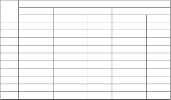
ERROR CALCULATION FOR x1 (t )
t Exact STHWS Leapfrog
0.1 1.569587765 1.569589365 1.6E-06 1.569587781 1.6E-08
0.2 1.698871678 1.698874878 3.2E-06 1.69887171 3.2E-08
0.3 1.684532785 1.684535685 2.9E-06 1.684532814 2.9E-08
0.4 1.625184166 1.625186366 2.2E-06 1.625184188 2.2E-08
0.5 1.553514795 1.553516195 1.4E-06 1.553514809 1.4E-08
0.6 1.480276073 1.480276973 9E-07 1.480276082 9E-09
0.7 1.408923352 1.408923552 2E-07 1.408923354 2E-09
0.8 1.340489359 1.340585359 9.6E-05 1.340490319 9.6E-07
0.9 1.275206129 1.275295129 8.9E-05 1.275207019 8.9E-07
1.0 1.213044618 1.213127618 8.3E-05 1.213045448 8.3E-07
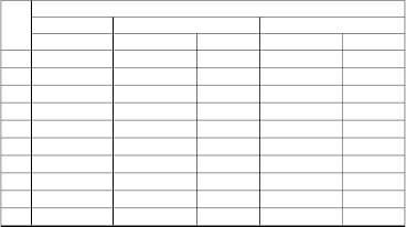
TABLE 2
ERROR CALCULATION FOR x2 (t )
where x is an n-state vector and A and B are
φ (t ) is an initial function.
n × n matrices.
t
And the singular delay system of the form is considered
Kx(t ) = Ax(t ) + Bx(t − h)+ Cu(t )
x(t ) = φ (t ) on [-h,0]
where K is an n × n singular matrix, A and B are n × n matrices
0.1 -0.618358341 -0.618356041 2.3E-06 -0.618358318 2.3E-08
0.2 -0.79403426 -0.79403156 2.7E-06 -0.794034233 2.7E-08
0.3 -0.823824809 -0.823821709 3.1E-06 -0.823824778 3.1E-08
and C is an
n × m
matrix. φ (t ) is an initial function, x is an n-
0.4 -0.806453413 -0.806449913 3.5E-06 -0.806453378 3.5E-08
state vector and u is an m-vector of control.
To highlight the efficiency of the Leapfrog method, we
consider the following two different examples taken from the
real world applications (4 Example and 5 Example), along
with the exact solutions. The discrete solutions obtained by the
two methods, Leapfrog method and STHWS method, the ab-
solute errors between them are calculated. To distinguish the
effect of the errors in accordance with the exact solutions, a graphical representation is given for selected values of “ x “and is presented in Figures 1 - 4 and Table 1 - 4 for stiff delay and singular delay systems, using three-dimensional
effect.
0.5 -0.774714012 -0.774710112 3.9E-06 -0.774713973 3.9E-08
0.6 -0.739457853 -0.739453553 4.3E-06 -0.73945781 4.3E-08
0.7 -0.704235263 -0.704230563 4.7E-06 -0.704235216 4.7E-08
0.8 -0.670169313 -0.670164213 5.1E-06 -0.670169262 5.1E-08
0.9 -0.637577977 -0.637572477 5.5E-06 -0.637577922 5.5E-08
1.0 -0.606513958 -0.606508058 5.9E-06 -0.606513899 5.9E-08
Consider the singular delay system S. Sekar et al. [6]
1 0 x1 (t )
− 1
0 x1 (t )
− π / 2e
0 x1 (t − 1)
1 0 0
Consider the stiff delay system S. Sekar et al. [6]
0 0 x (t ) = − 1
1 x (t ) + 1
0 x (t − 1) + 0
1
2
2
2
1
x1 (t )
11
21 x1 (t )
q − 2 p
2 p − 2q x1 (t − 1)
with x(t ) = [1
e −1]T
on [−1
0]. The exact solution of (6) is
x (t ) = − 21 / 2
− 41 / 2 x (t ) + p − q
p − 2q x (t − 1)
2
2
2
x1 (t ) = exp(− t )sin(πt / 2)
x2 (t ) = exp(− t )sin(πt / 2) + exp(− t + 1)cos(πt / 2) − 1
IJSER © 2013
http://www.ijser.org
International Journal of Scientific & Engineering Research, Volume 5, Issue 12, December-2014 1252
ISSN 2229-5518
the discrete time solution and the exact solution are evaluated. The results are shown in Table 3-4 and Fig. 3-4.
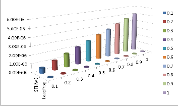
FIG. 1. ERROR ESTIMATION OF EXAMPLE 4 AT
x1 (t )
FIG. 2. ERROR ESTIMATION OF EXAMPLE 4 AT x2 (t )
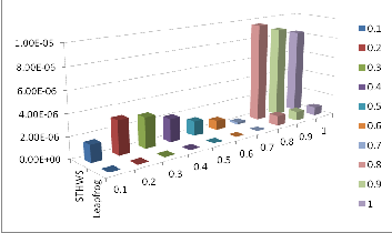
FIG. 3. ERROR ESTIMATION OF EXAMPLE 5 AT
x1 (t )
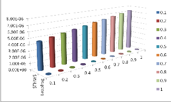
TABLE 3
ERROR CALCULATION FOR x1 (t )
t Exact STHWS Leapfrog
FIG. 4. ERROR ESTIMATION OF EXAMPLE 5 AT x2 (t )
0.1 0.372900226 0.372904826 4.6E-06 0.372900272 4.6E-08
0.2 -0.614856354 -0.614851454 4.9E-06 -0.614856305 4.9E-08
0.3 0.708500714 0.708505914 5.2E-06 0.708500766 5.2E-08
0.4 -0.664809247 -0.664803747 5.5E-06 -0.664809192 5.5E-08
0.5 0.516099076 0.516104876 5.8E-06 0.516099134 5.8E-08
0.6 -0.306669932 -0.306663832 6.1E-06 -0.306669871 6.1E-08
0.7 0.083106381 0.083112781 6.4E-06 0.083106445 6.4E-08
0.8 0.114050189 0.114056889 6.7E-06 0.114050256 6.7E-08
0.9 -0.256093348 -0.256086348 7E-06 -0.256093278 7E-08
1.0 0.328882993 0.328890293 7.3E-06 0.328883066 7.3E-08
TABLE 4
ERROR CALCULATION FOR x2 (t )
t Exact STHWS Leapfrog
0.1 -2.868118601 -2.868118001 6E-07 -2.868118595 6E-09
0.2 -0.145294494 -0.145293394 1.1E-06 -0.145294483 1.1E-08
0.3 -0.879794603 -0.879793003 1.6E-06 -0.879794587 1.6E-08
0.4 -1.897974291 -1.897972191 2.1E-06 -1.89797427 2.1E-08
0.5 0.382208613 0.382211213 2.6E-06 0.382208639 2.6E-08
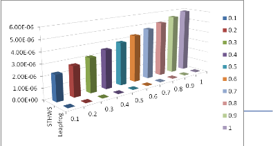
The obtained discrete solution of the numerical examples shows the efficiency of the Leapfrog method for solving the stiff delay and singular delay systems. From the Figures 1 - 4, we can observe that for most of the problems, the absolute error is less (almost no error) in Leapfrog method when com- pared to the STHWS [6] which yields a little error, along with the exact solutions. From the Figures 1 - 4 and Tables 1 - 4, one can predict that the error is very less in Leapfrog method when compared to STHWS method [6]. Hence, the Leapfrog method is more suitable for studying the stiff delay and singu- lar delay systems.
IJSER © 2013 http://www.ijser.org
International Journal of Scientific & Engineering Research, Volume 5, Issue 12, December-2014 1253
ISSN 2229-5518
[1] G.A. Bocharov, G.I. Marchuk and A.A. Romanyukha, “Numerical solution by LMMs of stiff delay differential systems modelling an immune response”, Numer. Math., vol. 73, pp. 131–148, 1996.
[2] L. Dai, Singular Control Systems, Springer-Verlag, 1989.
[3] E. Grispos, G. Kalogeropoulos and I. G. Stratis, “On generalized line- ar singular delay systems”, J. Math. Anal. Appl., vol. 245, pp. 430–446,
2000.
[4] S. Karunanithi, S. Chakravarthy and S. Sekar, “Comparison of Leap- frog and single term Haar wavelet series method to solve the second order linear system with singular-A”, Journal of Mathematical and Computational Sciences, vol. 4, no. 4, pp. 804-816, 2014.
[5] S. Karunanithi, S. Chakravarthy and S. Sekar, “A Study on Second- Order Linear Singular Systems using Leapfrog Method”, International Journal of Scientific & Engineering Research, vol. 5, pp. 747-750, 2014.
[6] S. Sekar and K. Jaganathan, “Analysis of the singular and stiff delay
systems using single-term Haar wavelet series”, International Review of Pure and Applied Mathematics, vol. 6, no. 1, pp. 135-142, 2010.
[7] S. Sekar and K. Prabhavathi, “Numerical solution of first order linear fuzzy differential equations using Leapfrog method”, IOSR Journal of Mathematics, vol. 10, no. 5, ver. I, pp. 07-12, 2014.
[8] S. Sekar and S. Senthilkumar, “A Study on Second-Order Fuzzy Dif- ferential Equations using STHWS Method”, International Journal of Scientific & Engineering Research, vol. 5, no. 1, pp. 2111-2114, 2014.
[9] S. Sekar and M. Vijayarakavan, “Numerical Investigation of first
order linear Singular Systems using Leapfrog Method”, International
Journal of Mathematics Trends and Technology, vol. 12, no. 2, pp. 89-93,
2014.
[10] J. Wei, The Degenerate Differential Systems with Delay, AnHui Univ.
Press, (1998), Hefei.
[11] J. Wei and Z. Zheng, “The general solution for the degenerate differ- ential system with delay”, ActaMath. Sinica, vol. 42, pp. 769–780,
1999.
[12] J. Wei and Z. Zheng, “The constant variation formula and the general solution of degenerate neutral differential systems”, Acta Math. Appl. Sinica, vol. 21, pp. 562–570, 1998.
[13] J. Wei and Z. Zheng, “The algebraic criteria for the all-delay stability of two-dimensional degenerate differential systems with delay”, Chi- nese Quart. J. Math., vol. 13, pp. 87–93, 1998.
[14] J. Wei and Z. Zheng, “On the degenerate differential systems with delay”, Ann. Differential Equations, vol.14, pp. 204–211, 1998.
[15] J. Wei and Z. Zheng, “The solvability of the degenerate differential systems with delay”, Chinese Quart. J.Math., vol. 15, pp. 1–7, 2000.
[16] J. Wei and Z. Zheng, “The V -functional method for the stability of degenerate differential systems with delays”, Ann. Differential Equa- tions, vol. 17, pp. 10–20, 2001.
[17] J. Wei, “Variation formula of time varying singular delay differential systems”, J. Math., vol. 24, pp. 161–166, 2003.
[18] J. Wei, “Eigenvalue and stability of singular differential delay sys-
tems”, J. Math. Anal. Appl., vol. 297, pp. 305–316, 2004.
IJSER © 2013 http://www.ijser.org