International Journal of Scientific & Engineering Research Volume 3, Issue 4, April-2012 1
ISSN 2229-5518
Numerical Simulation of Non-Premixed
Turbulent Methane-Air Combustion.
O.A Erinfolami, O.S Ismail, O. Oyewola
Abstract: This paper examined the heat-transfer coefficients and the Nusselt number for turbulent flow for a methane-air flame occurring in cross-flow streams in an open duct. The governing equation of momentum, energy, mass fraction and radical nuclei concentration were solved in a fully coupled fashion at each control volume. The model encompasses conservation equations of gas components participating in the process and energy equation. A FORTRAN code was written with a Tridiagonal matrix solver (TDMA) used to obtain the temperature, velocity and particulates profiles on the flat plate. The Nusselt number for the flow was calculated and plotted as a function of the calculated Rayleigh number. It was observed that a curve obtained with temperature and pressure far from the critical region approaches the line obtained with a classic correlation.
Index Terms— Computation Fluid Dynamics, Eddy dissipation model, Large eddy simulations, Non-Premixed combustion, Probability
Density Functions, Reynolds stress model, Reynolds Averaged Navier-Stokes, Turbulence,.
—————————— ——————————
1 INTRODUCTION
early all methods of engineering power production in- volve fluid flow and heat transfer as essential processes. The same processes governed the heating and air-
conditioning of buildings. Major segments of the chemical and metallurgical industries use components such as furnaces, heat exchangers, condensers, and reactors (nuclear), where thermo-fluid processes are at work. Aircrafts and rockets movements owe much too to fluid flow, heat transfer, and chemical reactions. In the design of electrical machinery and electric circuits, heat transfer is also often the limiting factor. The pollution of the natural environment is largely as a result of heat and mass transfer activities. Similarly are storms, floods, fires and some other natural events. Due to change in weather conditions, the human body resorts to heat and mass transfer for its temperature control.
Combustion is one of the oldest technical processes, and is an everyday phenomenon. It is the dominant mode of energy conversion. Today, combustion related researches are driven mainly by three objectives: Obtaining maximum effi- ciency, with an eye on the limited supply of fossil fuels; mini- mizing pollution to preserve the environment and achieving safe and stable operation of machinery and equipments.
The main challenge for combustion researchers, how- ever, is to accomplish all these goals simultaneously. Turbu- lent non-premixed flames exhibit phenomenon found in other turbulent fluid flows. In some circumstances a thin flame sheet forms a connected but highly wrinkled surface that separates the reactants from the products. This flame surface is con- vected, bent, and strained by the turbulence and propagates (relative to the fluid) at a speed that can depend on the local conditions (surface curvature, strain rate, etc.). Typically, the specific volume of the products of combustion is seven times that of the reactants, the flame surface being a volume source. Because of this large volume source there is a pressure field associated with the flame surface that affects the velocity field and hence indirectly affects the evolution of the surface itself.
Looking at the detailed structure of a turbulent non- premixed flame, we can examine mean quantities. Within the
flame there is a mean flux of reactants due to the fluctuating components of the velocity field. Contrary to normal expecta- tions and observations in other flows, it is found that this flux transports reactants up the mean-reactants gradient, away from the products (hence counter gradient diffusion).
A second notable phenomenon is the large produc- tion of turbulent energy within the flame: Behind the flame the velocity variance can be 20 times its upstream value. Both of these phenomena result from the large density difference be- tween reactants and products and from the pressure field due to volume expansion. There is a wide variety of theories and models for premixed and non-premixed turbulent flames. More ambitious are the probabilistic field theories that attempt to calculate statistical properties of a flame as functions of po- sition and time. In non-premixed flames, also called diffusion flames, the fuel and the oxidizer are mixed during the com- bustion process itself. Both premixed and non premixed flames can further be classified as either laminar or turbulent depending on the regime of gas flow.
There is an extensive literature describing the devel- opment of modeling techniques suitable for large-scale engi- neering simulations. Early studies of this type using single step chemistry were performed by [1], [2]. More recently, [3] have performed direct numerical simulations of turbulent, premixed hydrogen flames in three dimensions with detailed hydrogen chemistry. Bell et al. [4] have performed similar Numerical Simulation of Premixed Turbulent Methane Com- bustion.Three different statistical techniques use in turbulent modeling are the Large Eddy Simulations (LES), Reynold Av- erage Navier-Stokes Simulations (RANS) and Probability Den- sity Function (PDF) transport equations model [5]. In LES, the volume-averaging of the governing equations is considered, but will require large computational resources for routine si- mulations. It is however considered to be a promising tool. RANS technique solves the governing equations by modeling both the large and the small turbulent eddies, taking a time – averaged of the variables being considered. The PDF transport equation model consist of a procedure considering the proba-
IJSER © 2012 http://www.ijser.org
International Journal of Scientific & Engineering Research Volume 3, Issue 4, April-2012 2
ISSN 2229-5518
bility distribution of the relevant stochastic quantities directly by means of probability density functions.
2.3.1 Continuity equation
2.0 MODEL.
2.1 Field Model.
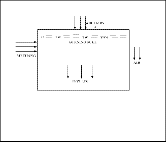
The schematic model of turbulent diffusion flame is as pre-

t
u 0
x j
(1)
sented in Fig 1. The overall effects of flame in the flow field has to be reduced to generation of heat and the dispersal of heat and burnt particules by either natural air or draughted air towards an object for heating. To carry out detail analysis of
Where uj is the jth Cartesian component of velocity and is
the fluid density. (j = 1,2,3)
2.3.2 Momentum equation
(2)
actions reflecting occurrences in the flow field a model of the flow field employing time averaged Navier–Stokes equations.
u
t
x i
u i u i

p
x i

ij
x i
f j
Where p is the static pressure, ij
is the viscous stress tensor
and fj is the body force. For Newtonian fluids ij can be ex-
pressed as:
u
i
u j
2
u k

ij x


x i

3 x k
(3)
Where is the fluid dynamic viscosity and necker delta
2.3.3 Energy Equation
ij
is the Kro-
The equation for the conservation of energy can take several forms. The static enthalpy form of the energy equation can be expressed as:
Fig 1 Problem simplified- schematic model of field for
h


u h qj p u

p

ui J h
(4)
study.
t xj
xj
j x
ij x
xj
mj m
2.2 Flame configuration and Field Definition.
For a two-dimensional parabolic flow, when a steady two- dimensional flow has one-way space coordinate, it is called a two dimensional flow. Most flame flow has a predominant
Where J mj is the total (concentration – driven + temperature – driven) diffusive mass flux for species m, hm represents the enthalpy for species m, and qj is the j – component of the heat flux. Jmj, hm and h are given as:
velocity in one way coordinate and hence the convection al- ways dominates the diffusion in that coordinate. It is this fea- ture that imparts the one way character to the stream wise direction. No reverse flow in this direction is acceptable. Ex-
J ij
D
T

Y m
X j
(5)
amples of two-dimensional parabolic flow are plane or axi- symmetric cases of boundary layers on walls, duct flows, jets, wakes, and mixing layers. The solution for such situation is
hm
Cp
T O
n
m T dT
h O f
(6)
obtained by starting with known distribution of the variable, Ф, at upstream station and marching in the streamwise direc- tion. For every forward step, the distribution of Ф in the cross
h
m 1
Y m h m
(7)
stream coordinate is calculated at on streamwise station. Thus
D is the diffusion coefficient, Cp is the constant – pressure spe-
O
computationally only one-dimensional problem needs to be
cific heat, and h f
is the enthalpy of formation at standard
handled, for which TDMA can be employed as solvers to the discretized equations of these variables Ф.
conditions PO 1.atm, ,TO 298K .
The Fourier’s law is employed for the heat flux:
2.3 Governing Equations.
Employing a conservative finite – volume methodology re- quires all the governing equations to be expressed in a con-
q n K
T
x j
(8)
servative form in which tensor notation is generally employed. The basic governing equations are for the conservation of
2.3.4 Mixture Fraction
f
mass, momentum and energy.
f
u
f D k
t
IJSER © 2012 http://www.ijser.org
x j
x j
x j
(9)
International Journal of Scientific & Engineering Research Volume 3, Issue 4, April-2012 3
ISSN 2229-5518
Where D is the diffusion coefficient, fk is the mixture fraction for the kth mixture.
2.3.5 Standard K - model expressed
For components A and B

Y YB A S
value of at a B rich inlet,
o
(18)
value of at a A
u k
k
(10)
rich inlet
t k
x
x
j
Pk
x j
For species A, reaction rate is expressed as
u j
C P C
2
(11)
t
x j
j
j
i k k
2 k
R A. . . min Y , YB
A k A S
, B Yc
1 S
(19)
Here P
T

u i S 2
(12)
k x T
S mixture wt of components B, The constants A = 4.0, B =
S= mean strain rate=
2Sij Sij
(13)
0.5, for micro mixing requirements
1
3 . k 1 n Sc Y 2
Pk – generation of turbulent due to buoyancy
m12 2
21
5.53
(20)
2.3.6 Chemistry /Reaction Model
The reaction model employed here for CFD development is the instantaneous chemistry model in which the reactants are
Further work (comprehensive energy calculations) Num flame
Total Energy in a chemical reaction is given by
2
assumed to react completely upon contact. The reaction rate is
E h P V h
sensible enthalpy ( 21)
infinitely rapid and one reaction step is assumed. Two reac- 2
tants, which are commonly referred to as “fuel” and “oxidiz-
er”, will be involved. A surface “flame sheet” separates the
h Y h p
T
Species i,

h i h
cp dT
two reactants (this assumption can be made only for non-
premixed flame).
The eddy dissipation model for the chemistry of reactions,
one step reaction model
i T i
Standard EDC model
For combustion reactions, a single step irreversible reaction with finite reaction rates
CH4 + 202  02 + 2H20
Methane activation energy E =48.0 cal/mole
A = the pre exponential factor = 8.3 X10¹⁶, hj – enthalpy of
1kgA SkgB 1 S kgC
(14)
component j in a mixture, Cp of mixture with temp variations,
S is the stochiometric mass requirement of species B to con- sume 1kg of A.
Mixture composition is determined by solving for only two
m - density of mixture
2.3.7 Heat and Mass Transfer Model
Transport Equation for energy can be written as
variables, mass fraction of specie A, YA and mixture frac-
E
E P
k
T
tion j . Using (13), above
t xi
i
x j
ef x S h
(22)
.
.u j Y A
T .
Y A
(15)

t Y A
and

x j


R A
j i j
Where E = total energy , Keff = effective thermal conductivity
C
Keff K p t
Prt

(23)
.Y
.u
T .
(16)
t A x
j j x
Sc
x
K – thermal conductivity of component, Turbulent diffusion
j j T j
coefficient ,
t

t 5
Where RA – tone averaged reaction rate. ScT- turbulent
Schmidt number, validity requires ScT to be same for all spe- cies.
- conserved combined variable
ct
Effective diffusion coefficient,
eff
t

0
(17)
3.0 THE SOLUTION PROCEDURE.
3.1 Developement Of The Simpler Algorithm.
IJSER © 2012 http://www.ijser.org
International Journal of Scientific & Engineering Research Volume 3, Issue 4, April-2012 4
ISSN 2229-5518
Once N avier – Stokes partial differential equations governing a flow field are formulated it is incumbent to develop the means of solving the equation. One of the popular methods in use is the method of procuring numerical solution via the SIMPLE algorithm. The procedure is as follows.
If is a variable and represented by a polynomial of the form, in x-direction
a p Tp aE TE a wTw a N TN as Ts b
(26)
= a + a x+ a x2+……….+ a x m
(24)
a 0 1 2 m
The unknowns
a0 , a1 , a2 ,...................., am are calculated by
treating the dependent variable x at a finite number of loca-
tions (the boundaries) on a grid of a chosen domain. The me-
thods involves the generation of a set of algebraic equations
for these unknowns and the prescription of an algorithm for solving the equation.
3.2 Control Volume Formulation.
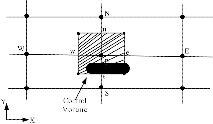
Fig. 2 – Two Dimensional Control Volume
Where
First we replace a given continuum with a grid formation of continuous discrete units over the given space, the flow field. The calculation domain is divided into a number of non –

a key , a
E xe w

k

w y
xw
overlapping control volumes such that there is one control
a k n x , a
k s x
volume surrounding each grid point. The differential equation
is integrated over each control volume. Piecewise profiles ex-

N
N

s
s
(27)
pressing the variation of between the grid points are used
o
cxy o o
to evaluate the required integrals. The result is the discretiza- tion equation containing the values of for a group of grid
a p

t , b Scxy a p T p
o
points. It is not compulsory that distancesbetween the grids
are equal. The use of non – uniform grid spacing is often de-
sirable, to deploy computer power effectively, we should note
that close to – accurate experimental results are obtained when
grid spacing are fine. The number of grid points that should
be distributed and numbers depend on the nature of problems
to be solved.
3.2.1 Boundary Condition.
The boundary conditions for the two dimensional flame mod- eling described below:.
(1) Symmetric centerline
a p QE aw a N as a p S p xy
3.2.3 Method of Solution of the Linear Algebraic Equa- tions
The solution of the discretization equation can be obtained by the Gaussian – Siedel iteration method. In a system with grids
1,2,3,………………., N with 1 and N being the boundary
points, the dicretization equation can be written as, for a vari-
able T
(2) Outlet: The outlet is modeled by means of a pressure out- let; this pressure is set to be atmospheric.
ai Ti
bi Ti i Ci Ti i d i
(28)
(3) Outlet or burner wall: Depending on the choice, this boun- dary is an outlet or a wall. When a free flame is modeled, this is a pressure outlet. When a flame in a box is modeled a burn- er wall is chosen.
(4) Burner wall: The burner wall is set to a constant tempera- ture, and a non-slip condition is used.
(5) Inlet: The inlet will be given by a velocity profile, using the determined profiles from the Fig 1.
3.2.2 Dicretization for Two Dimensions.
We shall assume the heat flux q obtained prevails over face area Δy x 1. Using similar assumptions for other faces, a dif- ferrential equation of the form
Showing Temp Ti is related to temperature Ti + i and Ti – i.
Effort is made to produce a matrix form of the derived equa- tions of any of the given variable and the matrix is subse- quently solved using a special form of Gauss-siedel iterative procedures called Tridiagonal algorithm. The method gives better results with one and two dimensional problems. Though convergence of the method is slow for large numbers of grid points, the accuracy could be very high. In order to speed up or slow down the changes from iteration to iteration in order to obtain quick convergence to solution, we employ a overrelaxation as speed up, underrelaxation as slow down. Use of underrelaxation is more common to avoid divergence. Overrelaxation is more employed in Gauss – Siedel procedure.
c T
k T
k T S
(25)
4.0 NUMERICAL SOLUTION
t
x
x
y
y
4.1 Inlet Data.
can be derived. This can be discretized, as
Methane is delivered through a horizontal orifice that did not
protrude into the flame control volume. Composition of gas is
as tabulated below.
IJSER © 2012 http://www.ijser.org
International Journal of Scientific & Engineering Research Volume 3, Issue 4, April-2012 5
ISSN 2229-5518
Table 1 Particulates Data.
It is assumed that a fuel of 86 % methane content delivered at about 15 m/s at 25o C /1bar via a 24’’ pipe (alternatively use mass flow rate for fuel estimates). Air current is in the range 3
– 10m/s at normal 1 bar and 27oC chosen for the study. One step reaction is assumed outward boundary condition applies to flows
4.2. Combustion model
The 2-D flow and mixing fields were resolved by the solution of the 2-D, axisymetric forms of the density-weighted fluid flow equations, supplemented with the k-ε model. Transport equations of several species are solved with equations for the mixture fraction and its variance. Solution of the transport equations is achieved using backward difference for first de- rivatives centered differencing for second derivatives with the upwind scheme for flow constants as developed by [6]. The solver employed is the one-way adaptive TDMA procedure as stated above.
The conservation equations of species mass fraction are transformed into the flamelet space. The flamelet equa- tions are solved in pre-processing. The stationary solution is stored in tables containing the profiles of temperature and mass fractions for all chemical species as function of the mix- ture fraction, its variance and the scalar dissipation rate. The coupling of chemistry and flow field is performed via the mix- ture fraction, its variance and the scalar dissipation which were provided from the flow field calculations. These values at each computational cell are used to extract mean scalar properties from the chemistry look up tables. The flow field properties are updated and iterations continue until conver- gence criteria are met. The governing equations are discretized using the finite volume method in an axisymmetric Cartesian coordinates. The Revised Semi-Implicit Method for Pressure Linked Equation, SIMPLER numerical scheme is used to han- dle the pressure and velocity coupling. The computational domain covers an area from 0 to 1.0 m in the axial direction and 0 to 0.40m in the radial direction. Totally 62(x) × 24(y) uni- form grids are used in the simulations. It has been checked that the further increase of grid number does not significantly influence the simulation results. The mass flow rate, total tem-
perature, turbulence intensity and hydraulic diameter are spe- cified for the inlet boundary. At the outlet region, outflow condition is assumed and the symmetry condition on the side boundary. Therefore each unknown will appear in more than one equation in the system, and these equations must be solved simultaneously to give all unknown quantities.
4.3 Grid Size and Mesh generation
A uniform size adaptive grid system is employed. Grid testing was carried out on a limited scale for different plate lengths and a grid size, the results was satisfactory as changes in results conform to expectations. It was ob- served that as grid size numbers increases the number of iterations required for convergence also increases consi- derably and beyond certain limit convergence to a solu- tion was not achieved.
4.4 Boundary Conditions
Boundary conditions at the inlet are given separately for the fuel stream at the central jet and the air stream cross-flow. The streams are considered to enter the computational domain as plug flow, with velocities calculated from their respective flow rates. The temperatures of fuel and air are specified. In con- formation with the conditions used the fuel flow rate is taken as 0.9517 kg/s and the air flow rate is calculated to be 3.7638 kg/s. The temperatures for both the streams at inlet are 300 K. The temperature for air is taken to be 300 K. The inlet veloci- ties were calculated from the respective mass flow rates and densities of air and methane fuel using mass transport equa- tions. No soot is considered to enter with the flow through the inlet plane. Considering the length of the computational do- main to be 1.0m x 0.4 m, the fully developed boundary condi- tions for the variables are considered at the outlet. In case of reverse flow at the outlet plane, which occurs in the case of buoyant flame, the stream coming in from the outside is con- sidered to be atmospheric air. Axi-symmetric condition was considered at the central axis, while at the wall a no-slip, adia- batic and impermeable boundary condition is adopted.
4.5 Stability Criteria and Convergence Conditions
The choice of the incremental time-step was done very careful- ly as it is directly related to the stability of the explicit scheme. The first criteria demands that pure advection should not con- vey a fluid element past a cell in one time increment as the difference equations consider fluxes only between adjacent cells. Hence the time increment should satisfy the following inequality. Solution use an under-relaxation factor of 0.2 - 0.5 to achieve quick convergence as suggested by previous scho- lars. The corrected velocity is employed to determine conver- gence of derived solution.
5.0 RESULTS AND CONCLUSIONS.
5.1 Results, Observations and Discussions.
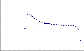
The results presented below revealed the events occurring in the visible forms of flame that we see. Flames are known to exhibit wavy pattern of flow due to recirculation currents found within its flow, this is shown by the negative values of particulates as seen in fig 2a and fig. 2b for the concentrates
IJSER © 2012 http://www.ijser.org
International Journal of Scientific & Engineering Research Volume 3, Issue 4, April-2012 6
ISSN 2229-5518
under consideration.
Methane Concentration at 0.03m
5.00E+11
0.00E+00
1 3 5 7 9 11 13 15 17 19 21 23
-5.00E+11
-1.00E+12
-1.50E+12
-2.00E+12
a x ia l positions
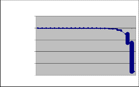
Fig 2a CH 4 particulate concentrations at 0.03m
2.00E+01
1.80E+01
1.60E+01
1.40E+01
1.20E+01
1.00E+01
8.00E+00
6.00E+00
4.00E+00
2.00E+00
0.00E+00
U- velocity at 0.03m
1 3 5 7 9 11 13 15 17 19 21 23
a x ia l position
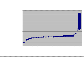
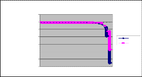
Fig 3b U-velocity distribution at 0.03m
O2 and C O2 C oncentration at 0.03m
2.00E+06
0.00E+00
-2.00E+06
-4.00E+06
-6.00E+06
-8.00E+06
-1.00E+07
-1.20E+07
1 4 7 10 13 16 19 22
a x ia l positi on
O2
CO2
5.00E+00
4.00E+00
3.00E+00
2.00E+00
0.00E+00
-1.00E+00
-2.00E+00
-3.00E+00
-4.00E+00
Fig 2b O2 and CO2 particulate concentrations at 0.03m
In some circumstances a thin flame sheet forms a connected but highly wrinkled surface that separates the reac- tants from the products.The flame surface is convected, bent, and strained by the turbulence and propagates (relative to the fluid) at a speed that can depend on the local conditions (sur- face curvature, strain rate, etc.) Further, the temperature (Fig
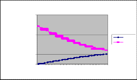
3a) shows definite increases as well as the u-velocity (Fig 3b). At this point the v-velocity (Fig 3c) of flow of methane gas/vapour begins to fluctuate rapidly this evidently suppor- tive of buoyancy effects accompanying temperature rise till the methane ignition temperature is reached.
a x ia l position
Fig 3c Velocity distribution at 0.03m.
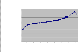
This rapidly changing v-velocity of methane as a re- sult of rapid temperature changes and resultant buoyancy continued beyond 0.1m till about 0.3m where stable positive values were obtained till the end of the control volume (Fig 4a and Fig 4b).
U- and V- velocity Distribution at 0.3m
2.50E+01
2.00E+01
Temperature Distributions at 0.03m
8.00E+02
7.00E+02
6.00E+02
5.00E+02
4.00E+02
3.00E+02
2.00E+02
1.50E+01
1.00E+01
5.00E+00
0.00E+00
1 4 7 10 13 16 19 22
a x ia l position
U-vel
V-vel
1.00E+02
0.00E+00
1 3 5 7 9 11 13 15 17 19 21 23
ax ial dista nce from e dge
Fig 4a Velocity distribution at 0.3m
Fig 3c Temperature distribution at 0.03m
IJSER © 2012 http://www.ijser.org
International Journal of Scientific & Engineering Research Volume 3, Issue 4, April-2012 7
ISSN 2229-5518
2.50E+03
Temperature at 0.3m
[4] Bell, J. B., , Day, M. S., and Grcar, J. F., Proc. Combust. Inst.,
29 (2002).
[5]Zegers R.P.C.,Flame stabilization of oxy-fuel flames, MSc.
Thesis, Eindhoven University of Technology. Report number
WVT 2007.13
[6] Patankar, S.V., Numerical Heat Transfer and Fluid Flow,
Taylor & Francis, Philadelphia / New York.. 1980.
2.00E+03
1.50E+03
1.00E+03
5.00E+02
0.00E+00
1 3 5 7 9 11 13 15 17 19 21 23
axi al position
Fig 4b Temperature distribution at 0.3m
One finds that the pollution of the solution with os- cillations is dependent on the domination of the convection terms over other terms of the differential equation, in practice most often diffusion terms in the governing transport equa- tions. The higher the Peclect and flow Reynolds numbers are, the more dominant is the convection term and the stronger is the pollution with oscillations.
As the cross wind velocity increases, a transition from buoyancy dominated flow to cross wind dominated flow can be noted along with a reduction in oscillation amplitudes.The changes of stability of flow begins to emerge in the diffusion flame leading to positive values showing that the v-velocity component profile presents in the flow is moving up. This effect is not only attributed to the buoyancy forces, but also due to the presence of the wall normal to the stream-wise di- rection. It is evident that the buoyancy forces have their im- pact in this region of the flame.
5.2 Conclusions.
A finite difference scheme for solving the fluid dynamic equa- tions of two dimensional elliptic flows has been used to pre- dict turbulent diffusion jet discharging perpendicularly into an unconfined cross-flow air current. The mathematical model employed a standard k-e model to calculate the distribution of Reynolds stresses. The turbulent gas phase, non-premixed combustion process was model using probability density func- tion approach assuming one step fast chemical reactions. Soot calculation was omitted in this study as its formation was con- sidered negligible. The purpose of the numerical model- ing/simulation on the turbulent diffusion flame is to deter- mine the profiles of variables and flow patterns for velocity, species concentration profiles, and temperature in the combus- tor area.
REFERENCES
[1] Trouve, A. and Poinsot, T., J. Fluid Mech., 278:1–31 (1994). [2] Zhang, S. and Rutland, C. J., Combust. Flame, 102:447–461 [3]Tanahasi, M.,Fujimura, M.,and Miyauchi,T.,Proc. Combust. Inst.,28:529–535 .2000.
IJSER © 2012 http://www.ijser.org