International Journal of Scientific & Engineering Research, Volume 5, Issue 4, April-2014 32

ISSN 2229-5518

Numerical Simulation of Air Velocity and

Temperature Distribution in an Office Room ventilated by Displacement Ventilation System

Qasim Hammodi Hassan*, Sabah Tarik Ahmed**, Ala'a Abbas Mahdi***

Abstract— In this study, a computational fluid dynamics (CFD) was used to simulate air velocity and temperature distribution fields for a three dimensional displacement ventilation system according to Iraqi climate. This study involved the solution of three dimensional partial differential equations for the conservation of mass, momentum, energy, turbulent energy and its dissipation rate. The finite volume method and the standard (k-ε) turbulence model were employed to solve the governing equations numerically.

A modified version of a three dimensional computer program FLUENT (6.3.26) was used to simulate the complex flow inside the room. The present computational program was validated by comparing the numerical results with experimental data of other study, This comparison show a good

agreement. Two main cases were studied with respect to the number of heat sources which were:-

1. Case I: Includes ventilated room with single heat source and one person.

2. Case II: Includes ventilated room with double heat sources and two persons.

The effect of ventilation rate corresponding to supply velocities (0.25–0.35 m/s) which is recommended by ASHRAE 2007, supply air temperatures

(17 & 19oC) and exhaust grille location on the thermal comfort were investigated based on air distribution performance index (ADPI) in the room.

For case I with a heat source of (50 W /m2) heat rejected, the ventilation rate is equal to (6.84 ACH), and supply air temperature of (19 oC) is needed to give better thermal comfort with ADPI equal to 83.6%. For case II with double heat sources each with (50 W /m2) heat rejected, (8.30 ACH) ventilation rate and supply air temperature of (19oC) were needed to get ADPI equal to 83.6%.

Keywords— CFD, Thermal comfort, Displacement ventilation.

——————————  ——————————

1 INTRODUCTION

he main aim of conditioning the interior environments of buildings is to provide a comfortable and healthy
indoor environment. Increasingly, concern is being expressed
over the quality of the indoor environment, where by failure
to provide satisfactory thermal conditions has resulted in
many reports of discomfort and ill health. As such, there has
been a constant need to study the thermal conditions of these indoor environments. Numerous studies have been conducted to explore the conditions of residential and commercial buildings, in which occupants spend large amount of their time every day.
The objectives of HVAC systems are to provide an acceptable level of occupancy comfort and process function, to maintain good indoor air quality (IAQ), and to keep system costs and energy requirements to a minimum [1].
In good health, the thermo-regulatory system of the body exercises automatic control over the deep tissue

temperature by establishing a correct thermal balance between the body and its surroundings. Apart from the matter of good health the comfort of an individual also depends on this balance and it might therefore be interpreted as the ease with which such a thermal equilibrium is achieved. ASHRAE Comfort Standard 55-74 goes further and defines comfort as '.. that state of mind which expresses satisfaction with the thermal environment..' but points out that most research work regards comfort as a subjective sensation that is expressed by an individual, when

* Eng. Qasim Hammodi Hassan, University of Technology, Machines and Equipment Dept, , Baghdad, Iraq.

** Prof. Dr. Sabah Tarik Ahmed, University of Technology, Machines and Equipment Dept, , Baghdad, Iraq.

*** Assist. Prof. Dr. Ala'a Abbas Mahdi, University of Babylon, Mechanical Engineering Dept., Babylon, Iraq.

questioned, as neither slightly warm nor slightly cool [2]. The
recommended temperature range inside the offices for better
thermal comfort between (23-26oC) [3].
Displacement ventilation increase the indoor air quality (IAQ) and saving energy in air conditioning and ventilation systems [4]. Displacement ventilation systems use very low discharge velocities, typically (0.25-0.35 m/s), to deliver cool supply air to the space. The discharge temperature of the supply air is generally above (16oC) [5]. The cool air is negatively buoyant compared to ambient air and drop to the floor after discharge. It then spreads across the lower level of the space and it is slightly heated as it passes over the floor surface. Buoyant plumes are developed around any warm objects in the room, such as people and electrical equipment. Each plume increases in width as it rises and entrains more air from the surrounding cooler air. This warm (and contaminated) air rises until it reaches an upper zone bounded by the ceiling.
The literature includes many investigations related to
the topic of ventilation inside an enclosure. Kobayashi. N and Chen. Q, (2003), studied the performance of a floor-supply displacement ventilation system using computational fluid dynamics (CFD), and demonstrates that, If the cooling load is high, the air change rate should be carefully selected to avoid a large temperature gradient [6]. Yukihiro Hashimoto, (2005), investigates airflow in an office room with a displacement ventilation system parametrically using three-dimensional CFD. The stratification profiles in the room depend especially on the supply air velocity [7]. Khudheyer S. Mushatet, (2006), used a two-dimensional turbulence (k-ε) model to predict the distribution of air velocity, temperature and turbulence kinetic energy in a ventilated room using different positions of inlet and outlet apertures [8]. Lau J. and Chen Q., (2007), reported the investigation of the performance of floor-supply

ER © 2014 http://www.ijser.org

International Journal of Scientific & Engineering Research, Volume 5, Issue 4, April-2014 33

ISSN 2229-5518

displacement ventilation with swirl diffusers or perforated panels under a high cooling load [9]. Z. Trzciakiewicz, (2008), presents the results of tests of the two-zone airflow pattern that forms in a room with displacement ventilation under condition of various heat sources and airflow rates [10]. Q.
Kong, B. Yu, (2008). Present a numerical prediction using
conservation of momentum). The equations are called Navier-Stokes equations, and for a three dimensional incompressible fluid take the form:
x-direction (U-momentum):

∂ ∂ ∂ ∂P ∂ ∂u ∂ ∂u ∂

( uu) + ( uv) + ( uw) = - + + +

∂x

computational fluid dynamics (CFD) utilized to investigate ∂u

∂y ∂z

1 ∂

∂x ∂x

∂u ∂v ∂w

∂x ∂y

∂

∂y ∂z

air temperature stratification in a room with an underfloor

�µ � +

∂z

�µ � + +

3 ∂x ∂x ∂y

�� +

∂z

(-ρu� ′�u�′) +

∂x

air distribution (UFAD) system [11]. J. Xaman et al.(2009),


(ρu� ′�v�′)+
(-ρu� �′w� �′)+ρgx (2)

∂y ∂z

presented a numerical study of conjugated heat transfer in a
ventilated cavity in order to analyze temperature distribution
y-direction (V-momentum):
effectiveness inside it, and four configurations for the outlet ∂ ∂ ∂

∂P ∂

∂v ∂

∂v ∂

of air were considered [12]. Kisup Lee et al. (2009), compared









(ρuv) + (ρvv) + (ρvw) = - + �µ � + �µ � +

∂x ∂y ∂z ∂y ∂x ∂x ∂y ∂y ∂z

the airflow, air temperature, and contaminant or air

�µ ∂v� + 1 ∂

�µ �∂u + ∂v + ∂w�� + ∂ (-ρu� ′�v�′)+
distribution effectiveness distributions in indoor spaces

∂z

∂ � � � ∂

3 ∂y

� � �

∂x ∂y ∂z ∂x

between the traditional displacement ventilation (TDV) and under-floor air distribution (UFAD) systems [13]. A. H. Taki et al. (2011), carried out experiments and CFD simulations to
(ρv′v′)+ (-ρv′w′)+ρgy (3)

∂y ∂z

z-direction (W-momentum):

∂ ∂ ∂

∂P ∂

∂w ∂ ∂w

test the use of a honeycomb slats system for suppressing








(ρuw) + (ρvw) + (ρww) = - + �µ � + �µ � +

∂x ∂y ∂z ∂z ∂x ∂x ∂y ∂y

downward cool air currents in a combined chilled

∂ �µ ∂w� + 1 ∂

�µ �∂u + ∂v + ∂w�� + ∂ (-ρu� �′w� �′)+
ceiling/displacement ventilation environment [14]. S. J. Rees ∂z ∂z

∂ ∂

3 ∂z

∂x ∂y ∂z ∂x

and P. Haves. (2013), studied the characteristics of
displacement ventilation and chilled ceiling panel systems by


(ρv� ′�w� �′)+

∂y ∂z

(-ρw� �′�w� ′)+ρgz (4)
making temperature and air flow measurements in a test chamber over a range of operating parameters typical of office applications [15].

2.1.3 Conservation of Thermal Energy: The following equation represents the transport of heat within the

flow field.
The numerical and experimental studies in the previous

∂ ∂ ∂

∂ ∂t

∂ ∂t ∂

section have emphasized the importance of displacement





(ρut) + (ρvt) + (ρwt) = �Γ � +

∂x ∂y ∂z ∂x ∂x

�Γ � +

∂y ∂y ∂z

ventilation system as provide a good indoor air quality. The aim of this paper is to evaluate the usefulness of CFD techniques in modeling room air flow. Using FLUENT (6.3.26) program to investigate the velocity and temperature distribution change with changing the ventilation rate, supply air temperature and exhaust grille location for an office room with different arrangement.

2 MATHEMATICAL FORMULATION AND NUMERICAL SOLUTION

2.1 Governing Equations

The conservation equations which govern the continuity, momentum and energy at constant density in a cartesian coordinate can be presented as follows:

2.1.1 Conservation of Mass: The change in mass flow within a control volume must be equal to the mass flow in minus the mass flow out through the control volume surfaces, since mass cannot be created or destroyed. This can be expressed mathematically for an incompressible fluid as:

�Γ ∂t � + ∂ �– ρu� ′�t�′� + ∂ �−ρv� ′�t�′� + ∂ �−ρw� �′�t�′� + St (5)

∂z ∂x ∂y ∂z

The terms – ρu� ′�t�′, −ρv� ′�t�′ and −ρw� �′�t�′ are the turbulent heat fluxes, St is a source term allowing for the rate of
thermal energy production [16].

2.2 Mathematical Model

FLUENT version (3.2.26) and GAMBIT software were used to create and grid the rooms geometries and then to simulate room air distribution for two main cases.
A turbulence model in CFD calculations is a computational procedure to close the system of mean flow equations (1) to (5) to enable numerical calculation of these equations. The task of a turbulence model therefore is to express the Reynolds stresses in equations (2) to (4) and the turbulent heat fluxes in equation (5) by a set of auxiliary equations (differential and/or algebraic) containing time- mean quantities of the flow [16].
The distribution of eddy viscosity throughout the flow domain must be established in order to calculate the
momentum and heat diffusion coefficients for turbulent


∂ (ρu) + ∂

∂x ∂y

(ρv) + ∂

∂z

(ρw) = 0 (1)
equations. This is the job of the turbulent model. The model used in the present work has been the most widely applied,
where u, v and w were the three components of velocity
corresponding to the x , y and z respectively.

2.1.2 Conservation of momentum (Navier–Stokes equations): The momentum equations that govern the flow of fluid are derived from Newton’s second law of motion (the

and is commonly referred as the standard k-ε model. The eddy viscosity at each grid point is related to values of turbulence kinetic energy (K) and the dissipation rate of turbulence energy (ε), [17]:

IJSER © 2014 http://www.ijser.org

International Journal of Scientific & Engineering Research, Volume 5, Issue 4, April-2014 34

ISSN 2229-5518

CD ρ K2

µ =

ε

(6)
Where CD is the empirical constant. The turbulent energy is defined by the fluctuation velocities:

K = 1 (�u�′�2� + v� ′�2 + w� �′2�) (7)

2

The local distribution of (K) and (ε) require the solution of
two additional transport equations, which are divided from the Navier-Stokes equation. The (K) transport equation is:

∂ (ρUK) + ∂ (ρVK) + ∂ (ρWK) = ∂ �µt ∂K� + ∂ �µt ∂K� +

∂x ∂y ∂z

∂x σk ∂x

∂y σk ∂y

∂ �µt ∂K� + G

− ρε (8)

∂z σk ∂z k

∂U 2

∂V 2

∂W 2

∂U ∂V 2

∂U ∂W 2

G = µ [2 �� �

∂x

2

+ � �

∂y

+ � � � + � + �

∂z ∂y ∂x

+ � + � +

∂Z ∂x

�∂V + ∂W� ] (9)

The ε equation is given by:







∂ (ρUε) + ∂ (ρVε) + ∂ (ρWε) = ∂ �µt ∂ε� + ∂ �µt ∂ε� +
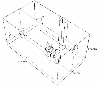
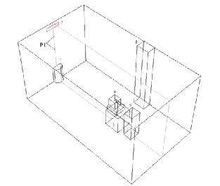
Fig (1). Schematic geometry of case I, (Plane P1at z=1.54m,

∂x ∂y ∂z

∂x σε ∂x

∂y σε ∂y

Plane P2 at y=0.35m)

∂ �µt ∂ε� + (C G

− C ρε) ε

(10)

∂z σε ∂z

1 k 2 K

Empiricism is introduced into the model through the five constants (C1, C2, CD, σk and σε) which are assigned the values given in table (3-1) [16 and 17].
Table (1) Constants of turbulence model

In the present study, the experimental test room, due to Ref. [15], was used as a case study model, the test chamber having internal dimensions of (5.43 m) long, (3.08 m) wide and (2.78 m) high. The displacement ventilation system air supply was via a semi-cylindrical diffuser (0.7 m) high and (0.4 m) diameter that is on the centerline of one of the shorter walls at low level.
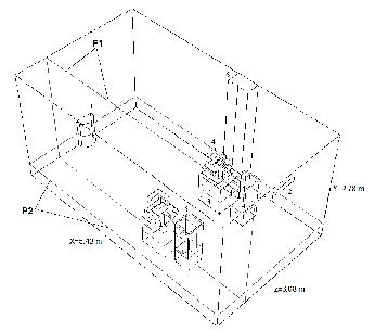
Also, in the current study, further complications like adding persons and solid tables with thermal boundary conditions according to climate of Iraq were investigated. Two main cases (Case I & Case II) were studied, respect to the number of heat sources which are, single heat source with one person and double heat sources with two persons respectively, (Figures (1 & 2)). The person was simulated with dimensions (0.35 m x 0.4 m x 1.1 m high), [18], and the table's dimensions were (0.6m x 0.6m x 0.72m high) [15].
Fig (2). Schematic geometry of case II, (Plane P1 at z=0.77m, Plane P2 at y=0.35m).
1-Diffuser air supply. 2- Exhaust grille. 3- Table. 4- Heat source. 5-Person. 6-Culomn.

2.3 Boundary Conditions

The boundary conditions for the model room are important in obtaining an accurate solution. Velocities at the walls are zero because of the no-slip condition. The no-slip boundary condition was also applied to the surfaces of the person, table and heat source. The table was assumed adiabatic because at steady state operation these surfaces will be at approximately the same temperature as the fluid surrounding them[19].
In order to obtain the thermal boundary conditions for CFD
simulation walls, floor and ceiling surfaces temperatures for

IJSER © 2014 http://www.ijser.org

International Journal of Scientific & Engineering Research, Volume 5, Issue 4, April-2014 35

ISSN 2229-5518

an actual room were measured with type "T" calibrated thermometer. The orientation of the actual room and measured data were applied on the room of case study to obtain a reliable simulation. The west and north walls are external walls while the east and south are internal walls. Table (2) shows the measured thermal boundary condition for walls, ceiling and floor. These boundary condition will used in all cases.
Table (2) Thermal boundary conditions.
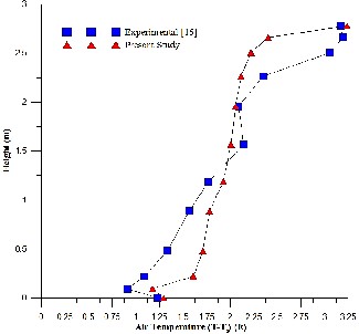
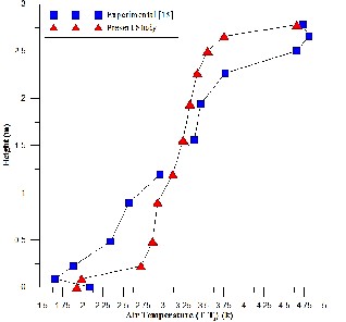
The comparison obtained a good agreement between the present work and published data. The difference between the experimental and numerical values is less than 16% for all cases.
Table (3) Boundary conditions and temperature distribution comparison for the validation cases of the
present work with published data, [15].

For all cases, the heat generated from the seating person will be (58.2 W/m2), [5].

2.4 Convergence Criteria

The prediction of flow is based on a solution of the fundamental flow equations. They consist of the equation of continuity, three momentum equations and the energy equation. The basic conservation equations for steady-state were solved by employing the finite volume, the second- order upwind scheme and the SIMPLE algorithm. The air was assumed to be incompressible and its physical properties were assumed constant, except that the air density was assumed to follow the Boussinesq approximation. The residuals of continuity, momentum, turbulence kinetic energy and its dissipation rate had to reach (1 x 10-4) magnitude for convergence, while the residual of energy had to reach (1 x 10-6) in magnitude.

3 VALIDATION

Since the CFD used approximation, it was necessary to validate the CFD program before it was used as a tool of study. The validation was done by comparing the CFD results with experimental data obtained in an environmental chamber with a wall-supply displacement ventilation system of Ref. [15] and tabulated in table (3).
The comparison depend on the vertical temperature
which measured by Ref. [15] in (12) locations and that of present numerical study. Figures (3) to (5) show the quantitative temperature distribution of the comparison.
The measured results were compared with the simulated results by using the overall average error calculations and absolute error due to the following equations,[20]:

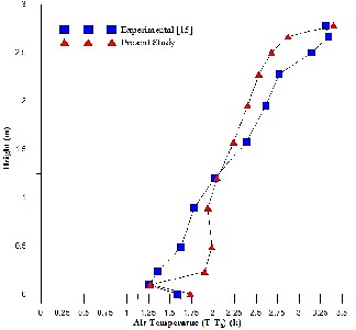
Fig.(3).Temperature distribution comparison in ventilated room for validation case (1).

n i −Ti �

∑i=1�TCFD

exp

E = i i

∗ 100% (11)

Where

∑i=1 Texp

n: number of measurements. T: air temperature (k).
Fig.(4).Temperature distribution comparison in ventilated room for validation case (2).

IJSER © 2014 http://www.ijser.org

International Journal of Scientific & Engineering Research, Volume 5, Issue 4, April-2014 36

ISSN 2229-5518

ACH = 3600∗Vin∗Ain

Vol.

(13)
Where:
ACH: air change per hour. Vin : velocity inlet (m/s).
Ain : net area of supply diffuser (m2). Vol.: net room volume (m3).
Table (4) Corresponding ventilation rates to the velocity ranges used in case I.

Fig.(5).Temperature distribution comparison in ventilated room for validation case (3)
.

4 INDEX FOR THERMAL COMFORT

The air distribution performance index was developed as a way to quantify the comfort level for a space air system in cooling. ADPI uses the effective draft temperature (EDT) collected at an array of points taken within the occupied zone to predict comfort. High ADPI values generally correlate to high space thermal comfort levels with the maximum obtainable value of 100%, [5].
The effective draft temperature (EDT) is given as, [16]:
EDT = (Tx - Tav) – 8*(Vx - 0.15) (12) Where
T x : local temperature (K)

Case II includes a ventilated room with two heat sources and two persons. Figure (2) shows the room of case II with the planes at which the graphic results where plotted (P1 & P2). The corresponding ventilation rates to the velocity ranges used shown in table (5), and it is calculated by equation (13).

Table (5) Corresponding ventilation rates to the velocity ranges used in case II.

5.1 Effect of Ventilation Rates

The ventilation rate for each case was studied for three flow rates equal to (6.84, 8.21 & 9.58) ACH for case I, (table (4)) and (6.92, 8.30 & 9.68) ACH for case II, (table (5)). The
T av : average room temperature (K)
temperature of inlet air in all three cases was equal to (17

oC)

Vx : local air velocity (m/s)
and the heat source give (50 W/m
). As a results, the cool
The effective draft temperature limit was taken as (1.1 K) for warm sensation and (-1.7 K) for cool sensation and the maximum air velocity was taken as 0.35 m/s. These values represent the limits for sedentary (office) occupation. The number of points at which the draft temperature satisfies the comfort limits above, expressed as a percentage of the total number of points, was defined as the air diffusion performance index (ADPI), [16].

5 RESULTS AND DISCUSSION

In the present study, the occupied zone was situated at
0.3 m from the sides walls, from the floor extended to 1.8 m
above the floor, [16]. Case I includes an office room with one heat source above a solid table and one person. The graphic results were plotted on the planes (P1 & P2) shown in figure (1). Table (4) shows the corresponding ventilation rates to velocity ranges used in case I according to the following equation:

2

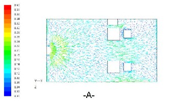
supply air drops and spreads across the floor and it is slightly heated as it passes over the floor surface. Figures (6) and (7) show the air distribution at plane P2 for the above two cases. Plane P2 for case I depicts that a good air distribution is reached, in case II a poor ventilation spot is formed behind the column.
There are slow air recirculation in the lower part of the
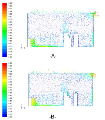
room ahead of the supply diffuser due to the horizontal air flow from the diffuser, as shown in figure (8). Figures (8) and (9) show the air distribution in plane P1 for each case with different ventilation rates. The cold air spreads through the floor of the room and then rises as the air warms due to heat exchange with heat sources in the room (people, heat source
& walls). The warmer air has a lower density than the cold air, and thus creates upward convective flows. Plumes are produced by convection as a result of difference in temperature between the air in contact with the heat sources and the surrounding air, it is clearly visible above the heat sources. The warm air then exits the room by extract grille in the upper part of the room.

IJSER © 2014 http://www.ijser.org

International Journal of Scientific & Engineering Research, Volume 5, Issue 4, April-2014 37

ISSN 2229-5518

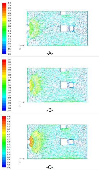
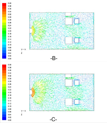
Fig (7). Air velocity distribution patterns for case II at plane
P2, Ts= 17oC.
VR= 6.92 ACH.
VR= 8.30 ACH.

VR= 9.68 ACH.
Fig (6). Air velocity distribution patterns for case I at plane
P2, Ts= 17oC.
A- VR= 6.84 ACH. B- VR= 8.21 ACH. C- VR= 9.58 ACH.

IJSER © 2014 http://www.ijser.org

International Journal of Scientific & Engineering Research, Volume 5, Issue 4, April-2014 38

ISSN 2229-5518

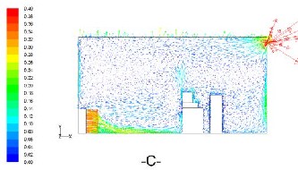
Fig (8). Air velocity distribution patterns for case I at plane
P1, Ts= 17oC.
A- VR= 6.84 ACH.
B- VR= 8.21 ACH.

C- VR= 9.58 ACH.
Fig (9). Air velocity distribution patterns for case II at plane
P2, Ts= 17oC. VR= 6.92 ACH. VR= 8.30 ACH.
VR= 9.68 ACH.
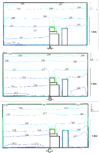
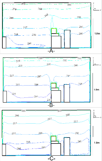
Since the cooling load was not changed, the total heat
removed by this system was same. Figures (10) and (11)
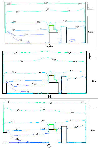
reveal the contour line of temperature distribution for the two mentioned cases at plane (P1). As a results, as the ventilation rate increase, it is clear that the vertical air temperature difference decreases due to increase the amount of delivered cold air to the room.

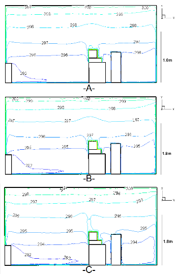
Table (6) show ADPI for the above two cases for a specified value of ventilation rate. ADPI change due to changing the air flow rate in the room with specified supply air temperature (17oC). Increasing the ventilation rate leads to increase the velocity of the air and decrease the vertical temperature difference which may be forms draft zone.
Fig (10). Temperature contours for case I, at plane P1 with
Ts=17oC.
A- VR= 6.84 ACH.
B- VR= 8.21 ACH.
C- VR= 9.58 ACH.

IJSER © 2014 http://www.ijser.org

International Journal of Scientific & Engineering Research, Volume 5, Issue 4, April-2014 39

ISSN 2229-5518

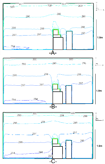
Fig (11). Temperature contours for case II, at plane P1 with
Ts=17oC.
VR= 6.92 ACH.
VR= 8.30 ACH.
AV= 9.68 ACH.
Table (6). ADPI for cases (I & II).
Table (6) shows that ADPI for case II needs a high ventilation rate than the other case due to high cooling load to reached ADPI equal to 81.7 %. While case I required a lower ventilation rate to reaches ADPI equal to 81.8%, both cases are with (50 W/m2) and supply air temperature (17oC).

5.2 Effect of Supply Air temperature

The effect of supply air temperature was studied with inlet air temperature equal to (17oC & 19oC) with three ventilation rates for each case. The previous section (5.1) was highlighted the velocity and temperature distribution of air in the cases (I & II) with inlet air temperature equal to (17 oC) and present section with supply air temperature (19 oC) with three ventilation rate for each case.
Figures (12) and (13) show the patterns of air
distribution for cases (I & II) with ventilation rate (8.21 &
8.30) ACH, respectively and supply air temperature (19 oC) at
plane P1. These figures indicate that the (2oC) temperature
difference in supply air temperature has no significant effect
on the air velocity in the room.

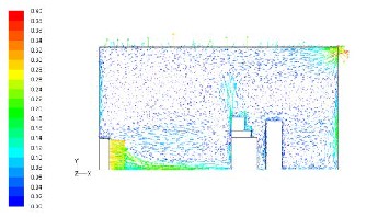
Fig (12). Air velocity distribution patterns for case I with 8.21
ACH, Ts=19oC and 50 W/m2.

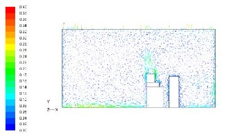
Fig (13). Air velocity distribution patterns for case II with
8.30 ACH, Ts=19 oC and 50 W/m2.
Displacement ventilation provides fresh air directly to the occupied zone. Therefore, the temperature distribution

IJSER © 2014 http://www.ijser.org

International Journal of Scientific & Engineering Research, Volume 5, Issue 4, April-2014 40

ISSN 2229-5518

compared to conventional mixing ventilation is sensitive to supply air temperature. Figures (14) to (15) depict the contour line of air temperature at plane P1 for cases (I & II) with different ventilation rates for each case. It is clear that increasing supply air temperature leads to increasing the vertical air temperature in the room.
ADPI depends on two parameters, local air velocity and
local air temperature. In present section, ADPI was not

effected with changing the supply air temperature by the air velocity since its change was not significant. The other parameter (local air temperature) has a great effect on ADPI due to the hot draft forms with increase the supply air temperature with low ventilation rate. Table (7) state ADPI values for cases (I & II) with supply air temperature (19oC) for given ventilation rate.
Fig (15). Temperature contour for case II with, Ts=19 oC and
50 W/m2.
VR= 6.92 ACH.
VR= 8.30 ACH. AV= 9.68 ACH.
Table (7) ADPI for cases (I & II).
Fig (14). Temperature contour for case I with, Ts=19 oC and
50 W/m2.
A- VR= 6.84 ACH.
B- VR= 8.21 ACH.
C- VR= 9.58 ACH.

IJSER © 2014 http://www.ijser.org

International Journal of Scientific & Engineering Research, Volume 5, Issue 4, April-2014 41

ISSN 2229-5518

Table (7) show that increasing supply air temperature with suitable ventilation rate and specified cooling load can be improving the thermal comfort. Lower temperature supply causes cold draft in the lower part of the room.

5.3 Exhaust Location

Case I was selected to study the effect of exhaust grille location on thermal comfort on occupied zone of displacement ventilation system. Case I was subdivided into three cases (a, b & c). In case (a), the extract grille was located on the east wall as shown in figure (1), in case (b), the extract grille was located on the ceiling as shown in figure (16), and in the case (c) the extract grille was located on the west wall as shown in figure (17).

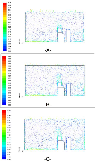
Figure (18) shows the air velocity distribution of cases
(a, b & c) in plane P1 with load (50 W/m2). The air velocity
distribution in occupied zone was same in all three cases and
the behavior of the air in the upper part of the room near the ceiling was changed.
Figure (19) shows the air temperature distribution contour of cases (a, b & c) with load (50 W/m2). When exhaust grille location was changed in case I the vertical air temperature distribution were almost the same in occupied zone. This is
because the upward air movement does not effected by the location of exhaust grill especially below (1.8 m) in occupied zone.

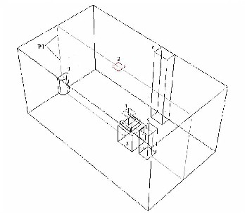
Fig (16). Schematic of room geometry of case (b).
Fig (17). Schematic of room geometry of case (c).

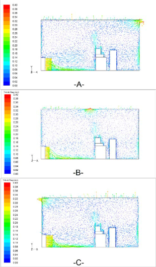
Fig (18). Air distribution patterns of cases (a, b & c) at 8.21
ACH, Ts=19oC & 50 W/m2.

IJSER © 2014 http://www.ijser.org

International Journal of Scientific & Engineering Research, Volume 5, Issue 4, April-2014 42

ISSN 2229-5518

Fig (19). Air temperature contour of cases (a, b & c) at 8.21
ACH, Ts=19oC & 50 W/m2.

6 CONCLUSIONS

In the present study, air velocity and temperature distribution fields in room with displacement ventilation system were numerically investigated. The simulation program was validated, and compared with experimental data of another researcher and shows a good agreement. The effect of ventilation rate supply air temperature and extract grille location on the thermal comfort was studied. We can conclude the following conclusions:
1. Standard (k-ε) turbulence model with SIMPLE
algorithm gives reliable results to simulate air velocity and
temperature distribution fields in displacement ventilation
system.
2. Higher ventilation rate and/or low supply air temperature is better for reducing the temperature gradient, but it may results in draft because of the higher supply air velocity.
3. The temperature gradient in the room were partially
large, since the cold and clean air from the supply diffuser stay in the occupied zone and do not mixed with the hot air in the upper part of the room.
4. The location of the exhaust grille in the upper part of the room (on ceiling or walls) has no effect on the thermal comfort in the occupied zone.

REFERENCES

[1] Samuel C. Sugarman, " HVAC Fundamentals" The Fairmont Press, Inc.2005.

[2] W.P. Jones, " Air Conditioning Engineering" Elsevier Butterworth-

Heinemann,5th edition, 2001 [3] Iraqi cooling codes, 2012.

[4] Laurent Magnier, Radu Zmeureanu and Dominique Derome," Experimental Assessment of the Velocity and Temperature Distribution in an Indoor Displacement Ventilation Jet", Building and Environment, Vol. 48, pp. 150-160, 2012.

[5] ASHREA, HVAC Aplications, 2007.

[6] Kobayashi, N. and Chen, Q, " Floor-Supply Displacement Ventilation in a Small Office", Indoor and Built Environment, 12, pp. 281-292, 2003.

[7] Yukihiro Hashimoto1, "Numerical Study on Airflow in an Office Room with a Displacement Ventilation System", Building Simulation, Ninth International IBPSA Conference, pp. 381-388,

2005.

[8] Khudheyer S. Mushatet, " Numerical Simulation of Turbulent Isothermal Flow in Mechanically Ventilated Room", JKAU: Eng. Sci., Vol. 17, No. 2, pp. 103-117, 2005.

[9] Josephine Lau and Qingyan Chen, " Floor-Supply Displacement Ventilation for Workshops", Building and Environment, Vol.42(2), pp.1-23, 2007.

[10] Z. Trzciakiewicz, " An Experimental Analysis of the Two Zone

Airflow Pattern Formed in Room with Displacement Ventilation" The International Journal of Ventilation Vol. 7, No.3, pp. 221-

231,2008.

[11] Qiongxiang Kong and Bingfeng Yu, " Numerical Study on Temperature Stratification in a Room with Underfloor Air Distribution System", Energy and Buildings, Vol. 40, pp. 495-502,

2008.

[12] J. Xaman, J. Tun, G. Alvarez, Y. Chavez and F. Noh, "Optimum Ventilation Based on the Overall Ventilation Effectiveness for Temperature Distribution in Ventilated Cavities", International Journal of Thermal Sciences. Vol. 48, pp. 1574-1585, 2009.

[13] Lee, K.S., Zhang, T., Jiang, Z., and Chen, Q., " Comparison of

Airflow and Contaminant Distributions in Rooms with Traditional Displacement Ventilation and Underfloor air Distribution Systems", ASHRAE Transactions, Vol. 115(2), 2009.

[14] A.H. Takia, L. Jalil and D.L. Lovedayc, " Experimental and Computational Investigation into Suppressing Natural Convection in Chilled Ceiling/Displacement Ventilation Environments Experimental and Computational Investigation into Suppressing Natural Convection in Chilled Ceiling/Displacement Ventilation Environments", Energy and Buildings, Vol.43, pp. 3082-3089, 2011.

[15] Simon J. Rees and Philip Haves, "An Experimental Study of Air

Flow and Temperature Distribution in a Room with Displacement Ventilation and a Chilled Ceiling " Building and Environment, volume 59, pp. 358-368, 2013.

[16] H. B. Awbi, “Ventilation of Buildings”, Spon Press, 2th edition,

2003.

[17] Ahmed Alaa'ddin Abduljabbar Al-Shawi, " Prediction of Radiant

Cooling Panels Performance in Mixed Convection Environments",

M.Sc. Thesis, University of Technology, 2012.

[18] Yan Huo, Ye Gao and Wan-Ki Chow, "Locations of Diffusers on Air

Flow Field in an Office", The Seventh Asia-Pacific Conference on

Wind Engineering, 2009.

[19] Senol Baskaya And Emre Eken, " Numerical Investigation Of Air

Flow Inside An Office Room Under Various Ventilation

Conditions", Journal of engineering Sciences, Vol. 12, Pp. 87-95,

2006.

[20] Johnson Lim Soon Chong, Adnan Husain & Tee Boon Tuan,

"Simulation of Airflow in Lecture Rooms", Proceedings of The

AEESAP International Conference, 7-8 June 2005.

IJSER © 2014 http://www.ijser.org