International Journal of Scientific & Engineering Research, Volume 5, Issue 1, January-2014 1977

ISSN 2229-5518

Nodally Integrated Finite Element Formulation for Mindlin-Reissner Plates

D. A. Simoes and T. A. Jadhav

Abstract— This work describes a nodally integrated finite element formulation for plates under the Mindlin-Reissner theory. The formulation makes use of the weighted residual method and nodal integration to derive the assumed strain relations. An element formulation for four-node quadrilateral elements is implemented in the nonlinear finite element solver Abaqus using the UEL user element subroutine. Numerical tests are carried out on the new element and the results are presented.

Index Terms— Abaqus, CAE, element formulation, finite element analysis, four-node quadrilateral element, nodal integration, UEL

——————————  ——————————

1 INTRODUCTION

N nodal integration, the numerical integration is carried out at the corner nodes of the element, rather than at quadrature points inside the element. Research on finite element formu- lations emerged in the beginning of the 1970s, while nodal integration in FEA is a relatively recent development, with the first works beginning in the year 2000 describing its applica- tion to tetrahedral elements. Wolff [1] discussed nodally inte- grated finite elements, focussing on solid elements. It was
Abaqus is an extremely capable nonlinear solver with a large element library that allows analysis of even the most complex structural problems. The default element formula- tions in Abaqus are accurate, robust and reliable enough, hav- ing been extensively tested. However, situations arise in which the Abaqus element library would not serve the pur- pose, and the user would like to define their own elements, such as:

IJSER

shown that nodally integrated elements show good conver-
gence compared to full integration when applied to incom-
pressible media. Nodal integration is also attractive because of
its applicability to meshfree methods as described by Quak et
al [2], who compared gauss integration and nodal integration for meshless analyses. This is because, as described in this formulation, the method focuses on a nodal patch, rather than on an elemental area, as conventional elements do. In large deformation processes, for example in extrusion and injection moulding, finite elements can suffer from excessive mesh de- formation. Meshless methods are well suited to avoid these problems. However, the obstacle that must be overcome in developing nodally integrated elements is that the quantities at nodal points are not continuous, and the nodes are shared among multiple elements. These elements also suffer from shear locking, being based on the Mindlin-Reissner theory for thick plates.
Wang and Chen [3] described a Mindlin-Reissner plate
formulation with nodal integration. Castelazzi and Krysl [4]
introduced Reissner-Mindlin plate elements with nodal inte-
gration in which the nodal integration is derived from the a priori satisfaction of the weighted residuals. They have ap- plied the same formulation, called the NIPE technique to a nine-node quadrilateral plate element [5]. However, in this case, a variational energy method is used instead of the weighted residual method in their previous work. The result- ing element is found to be an improvement over the earlier one. Giner, E. et al [6] and Park, K. et al [7], have implemented special elements for fracture mechanics in Abaqus UEL.

————————————————

D. A. Simoes and T. A. Jadhav,

Department of Mechanical Engineering, Sinhgad College of Engineering, University of Pune, India

• Modelling non-structural physical processes that are
coupled to structural behaviour
• Applying solution-dependent loads
• Modelling active control mechanisms
• Studying the behaviour of proposed formulations
For example, elements can be developed to function as con-
trol or feedback mechanisms in an analysis that consists of
regular elements. Moreover, it is easier to maintain and port a
subroutine than to do the same for a complete finite element
program.
The following are some desirable reliability criteria for fi-
nite element formulations [8]:
1. The element formulation must not incorporate nu-
merically adjusted factors which can be adjusted to make the
element accurate for one class of problems, but not for other
types of problems.
2. The element formulation must not contain spurious
rigid body modes.
3. The element should not lock in thin plate / shell anal-
yses.
4. The element formulation must satisfy patch tests.
5. The element accuracy should be insensitive to ele-
ment distortions and changes in material properties.
In this paper, we describe an element formulation which
makes use of nodal integration and the weighted residual
method to derive the assumed strain operators. This is applied to two elements: a four-node quadrilateral element and a three-node triangular element. A four-node quadrilateral ele- ment is then implemented in the nonlinear finite element solv- er Abaqus by writing a user element subroutine (UEL). In sec- tions 3 and 4, we follow the same procedure described in [4].

The research paper published by IJSER journal is about Nodally Integrated Finite Element Formulation for Mindlin-Reissner Plates 1978

ISSN 2229-5518

2 BASIC GOVERNING EQUATIONS

In this section, the basic equations of a Reissner-Mindlin
The curvatures and transverse shear strains are given by
𝜃𝑦,𝑥
plate theory are summarised. We denote the domain of the
𝜼𝑏 = �
𝜃𝑥,𝑦
� (5)
plate, which is its volume by V and the thickness by t.
𝑉 = {(𝑥, 𝑦, 𝑧) ∈ ℝ3| z ∈ [-t/2; t/2], (x,y) ∈ A ∈ ℝ2} (1)
−𝜃𝑦,𝑦 + 𝜃𝑥,𝑥
−𝜃𝑦 − 𝑤,𝑥
where A is the area of the plate and C=𝜕𝜕 is its boundary.
The Cartesian components of the displacement in three-
𝜼𝑠 = �

𝑥

− 𝑤,𝑦
� (6)
dimensional space are
𝑢𝑥 = z𝜃𝑦 , 𝑢𝑦 = −𝑧𝜃𝑥 , 𝑢𝑧 = 𝑤 (2)
The compatibility equations can be written as
bending strains,
𝜃𝑦 and 𝜃𝑥 are the rotations of the midsurface normal about
the Cartesian x and y axes and w is the displacement in z. The
curvatures,
𝜺𝑏
= 𝑧𝜷𝑏 𝒖� (7)
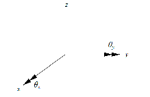
functions 𝜃𝑦 , 𝜃𝑥 , 𝑢𝑧 are the unknowns that we would like to determine. This is shown in Figs. 1 and 2. 𝜃𝑧 is the drilling de-
gree of freedom.
𝜼𝑏 = 𝜷𝑏 𝒖� => 𝜺𝑏 = 𝑧𝜼𝑏 (8)
shear strains,
𝜺𝑠 = 𝜷𝑠 𝒖� = 𝜸 = 𝜼𝑠 (9)
where 𝜷𝑏 and 𝜷𝑠 are the gradient matrices
The constitutive equations for plane stress
for bending,

for shear,
𝝈𝑏 = 𝑫𝑏 𝜺𝑏 = 𝑧𝑫𝑏 𝜼𝑏 (10)
𝝈𝑠 = 𝑫𝑠 𝜺𝑠 = 𝑘𝑘𝜼𝑠 (11)

Fig. 1. Notation for rotation components of a midsurface normal

For a homogeneous, linear elastic and isotropic material,

IJSER

Mindlin plate theory assumes that transverse shear defor- mation occurs, and the strains are given as follows:
𝐷 𝑣𝐷 0

𝑏 𝑣𝐷 𝐷 0

(1 − 𝑣)𝐷
� (12)

0 0

𝜀 = 𝜕𝜃𝑦 2
𝜀𝑦 = -z

𝜕𝑥

𝜕𝜃𝑥

𝜕𝑦

Here, the bending rigidity

𝐷 =
𝐸𝑡 3
(13)

𝛾 = 𝑧 �𝜕𝜃𝑦

𝑥𝑦 𝜕𝑦

− 𝜕𝜃𝑥 �
𝜕𝑥
12(1 − 𝑣 2 )

E is the Young’s modulus and ν is the Poisson’s ratio,

𝛾𝑦𝑧 = 𝜕𝑤�𝜕𝑦 − 𝜃𝑥
𝑫𝑠 = 𝑘𝑘𝑡 �1 0
1
(14)
𝛾𝑧𝑥 = 𝜕𝑤�𝜕𝑥 − 𝜃𝑦 (3)

G is the shear modulus. k is the shear correction factor, which accounts for the parabolic z-direction variation of the transverse shear stress, and kt can be regarded as the effective thickness for transverse shear deformation. It is taken to be

5/6 throughout.
The plate is loaded by boundary load 𝒃� = [0, 0, 𝑏�
(x,y)] T
The balance equation obtained after integrating through the
thickness of the plate is
𝜷𝑏𝑇 𝑴 + 𝜷𝑠𝑇 𝑺 + 𝑡𝒃� = 𝟎 (15)
and the resultants,

Fig. 2. Moments and transverse shear forces on a differential element of a

𝑡/2

−𝑡/2

plate

We express the three-dimensional displacement vector in terms of the mixed component vector of the generalised dis-
placements 𝒖�
𝝈𝑠 𝑑𝑧 = 𝑡𝑘𝑘𝜼𝑠 𝑫𝑠 𝜼𝑠 (17)

−𝑡/2

3 WEIGHTED RESIDUAL FORMULATION

𝒖� = [𝑤, 𝜃𝑥 , 𝜃𝑦 ]T (4)
The method of weighted residuals is applied to obtain the
weak form of the Mindlin-Reissner governing equations. The weak form will be constructed in a manner that facilitates a

The research paper published by IJSER journal is about Nodally Integrated Finite Element Formulation for Mindlin-Reissner Plates 1979

ISSN 2229-5518

locking-free FE discretisation.
Nodal quadrature cannot directly process the integrands
We obtain
� 𝑩� 𝐼
𝑫𝑠 �𝑩�𝐽 𝐽
from the individual elements to which the node is common,

𝑠𝑇

𝐴

𝑠 − 𝑩𝑠 �𝑑𝜕 = 0 ∀𝐽 (23)

because each contributing basis function derivative will be
multi-valued at the node (discontinuous across the element
edges). For the process of nodal quadrature, the basis func-
tions derivatives, or, equivalently, the strains should be com- puted using a special strain-displacement operator, so we use an assumed-strain method.
A separate residual statement is kept for each weakly en- forced boundary condition. The three residual equations are as
follows:
• The balance equation residual:

𝑇 𝑇

Fig. 3 explains the indices. For a particular I, we note that in order to formulate strictly local operations, we should only
consider the strain-displacement matrices 𝑩𝐽 defined within
the elements er , r = 1, … , 5 connected to node I. The index J

then ranges over J = Jq , q = 1, … , 6 and J = I. Therefore, we

replace ∀𝐽 in (23) with the limited range J ∈ nodes(elems(I)) ;
the term nodes(e) refers to nodes of the element e, the term
elems(I) refers to the elements connected to the node I, and the
term nodes(elems(I)) refers to the union of the nodes of the elements connected to the node I. Therefore we use the inte-
grals
𝑟𝐵 = ∫ 𝜼�𝑇 �𝜷𝑏 𝑴 + 𝜷𝑠 𝑺 + 𝑡𝒃��𝑑𝜕 = 0 (18)
• The natural boundary condition residual :
� 𝑩� 𝑠𝑇

𝐼

𝐴

𝑫𝑠 �𝑩� 𝑠 − 𝑩𝑠 �𝑑𝜕 = 0 (24)

𝐽 𝐽

J ∈ nodes(elems(I))

𝑟𝑐 = � 𝜼�1 (𝑆𝑛𝑧 – 𝑆𝑛𝑧 )𝑑𝑑 + � 𝜼�2 (𝑀𝑛𝑛 – 𝑀�𝑛𝑛 )𝑑𝑑
for any particular node I.

𝐶 ,1

𝐶 ,2

+ � 𝜼�3 (𝑀𝑛𝑠 − 𝑀�𝑛𝑠 )𝑑𝑑 = 0 (19)

𝐶 ,3

• The kinematic equation residuals:
𝑟𝐾𝑏 = � (𝜷� 𝑏 𝜼�)𝑇 𝑫𝑏 �𝜷� 𝑏 𝒖� − 𝜷𝑏 𝒖��𝑑𝜕 = 0 (20)

𝐴

𝑟𝐾𝑠 = � (𝜷� 𝑠 𝜼�)𝑇 𝑫𝑠 �𝜷� 𝑠 𝒖� − 𝜷𝑠 𝒖��𝑑𝜕 = 0 (21)

𝐴

Here 𝜼� is the test function (generalised displacement, as in-
dicated by the tilde ‘~’ ), which is assumed to vanish along the
portions of the boundary where essential boundary conditions are prescribed, in order to eliminate the unknown reactions:
[𝜼�]𝑖 = 0, where the ith component of the generalised dis-
placement is prescribed on C.
Next, the assumed strain operators 𝜷� 𝑏 and 𝜷� 𝑠 will be de-
rived from condition that they will make the kinematic resid-
uals (20) and (21) identically zero. The process will be the
same for both 𝜷� 𝑏 and 𝜷� 𝑠 . Hence, we will describe the deriva- tion of 𝜷� 𝑠 only.

4 PATCH AVERAGED ASSUMED STRAIN

We now derive the strain-displacement assumed-strain matri- ces for meshes of isoparametric three-node triangles, four- node quadrilaterals, or possibly a combination of both element types.
We introduce the finite element approximation 𝒖� = ∑𝐼 𝑁𝐼 𝒖� 𝐼
and 𝜼� = ∑𝐼 𝑁𝐼 𝜼�𝐼 .

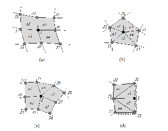
Fig. 3. Nodal patch illustrated on (a) four-node quadrilateral mesh; (b) three-node triangular mesh; (c) mixed mesh; and (d) a three-node triangu- lar mesh with boundary conditions

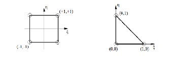
Fig. 4. Nodal quadrature locations for the triangular and quadrilateral ele- ments

Fig. 4 shows the quadrature rules for two of the simplest el-
We have introduced matrices 𝑩𝑠 = 𝜷𝑠
�𝑁𝐽 � and the strain-
ement formulations discussed. The weights are 1/3 for each
displacement matrices 𝑩� 𝐼 (not yet specified), that are used to
obtain the assumed strains as
node of a triangular element and 1 for each node of quadrilat- eral elements. Using numerical quadrature, the integral (24) is replaced by the following double sum:
𝜸 = � 𝑩� 𝐼 𝒖� 𝐼

𝐼

(22)

The research paper published by IJSER journal is about Nodally Integrated Finite Element Formulation for Mindlin-Reissner Plates 1980

ISSN 2229-5518

� � ℐ(𝒙 )𝑊 [𝑩� 𝑠𝑇
𝑫𝑠 (𝒙𝐾 )] = 𝟎
(25)
ratio ν. This is done through the command *UEL PROPERTY [11]. Since there is no way to display user elements in post-

𝑒 𝐾 ∈𝑛𝑜𝑑𝑒𝑠(𝑒)

J ∈ nodes(elems(I))

processors, all the user elements are duplicated with overlay elements with a very low stiffness. This enables the displace-
where e ranges over all the elements in the mesh, K ranges
over all the quadrature points in the element. Here, the quad- rature points coincide with the nodes. xK is the location of the
quadrature point (node), ℐ(𝒙𝑘 ) is the Jacobian of the isopara-
metric mapping, and WK is the weight of the quadrature point.
Finally we are led to the definition of the assumed-strain nodal matrix as a weighted average of the elemental strain displacement matrices.
ment to be visualised in the post-processor.
𝑩�𝐽

∑𝑒∈𝑒𝑙𝑒𝑚𝑠(𝐾) ℐ(𝒙𝑘 )𝑊𝐾 𝑩𝑠 (𝒙𝐾 )
∑ ℐ(𝒙 )𝑊

(26)

𝑒∈𝑒𝑙𝑒𝑚𝑠(𝐾)

𝑘 𝐾

Thus, constructing the nodal strain-displacement matrices
as averages of the strain-displacement matrices from the con- nected elements will satisfy the kinematic residual statement, enabling nodal quadrature in the process. If the integration point K lies at a multi-material interface, the above derivation is not valid since the material stiffness matrix Ds is multi- valued at xK . Under these circumstances, one must split the sum of the elements into two or more groups, one for each material. Then for each group, the material stiffness matrix
will be single-valued.
Since the element is integrated at the nodal points, the same
function can be used to interpolate the quantities within the
element as well as to describe the deflection. Thus, the element is an isoparametric element.

5 ABAQUS IMPLEMENTATION

In this section, the main features related to the Abaqus imple- mentation through the user subroutine UEL are discussed. The following information must be passed on to Abaqus from the user element code [9]:
 Strain – displacement matrix B
 Constitutive law matrix D
 Element stiffness matrix k
k=∫ 𝑩𝑇 𝑫𝑩𝑡𝑑𝑉
 Element internal force vector Fi
(27)
𝑭𝑖 = ∫ 𝑩𝑇 𝝈𝑑𝑉 (28)
 Numerical integration
These have to be coded in FORTRAN. In the subroutine,
nodal coordinates (COORDS), nodal displacements in the glob- al coordinates (U) and the material properties defined in the input file (PROPS) are available, while the right-hand-side vec- tor (RHS) and the Jacobian matrix (AMATRX) of an element need to be defined. In addition, the state dependent variables (SVARS) can be updated at the end of each iteration.
Each element has four nodes, and each node has three de- grees of freedom (w, θx, θy). First, the global nodal displace- ments are converted into local displacements.
Through the *USERELEMENT command, we define 4-node
user elements. We also provide three real-valued user proper-
ties: the element thickness t, Young’s modulus E and Poisson’s

Fig. 5. Global flow in Abaqus

The name of the FORTRAN file containing the UEL code must be added to the normal command for launching an Abaqus job as follows:

abaqus job=<job-id> user=<name-of-file>

Example:

abaqus job=clamped_strip.inp user=NIP-Q4.for

User elements in Abaqus cannot form part of a contact sur-
face. However, this problem can again be solved by making
use of the duplicate overlay elements to define the contact

The research paper published by IJSER journal is about Nodally Integrated Finite Element Formulation for Mindlin-Reissner Plates 1981

ISSN 2229-5518

surface. In addition, it is necessary to make some simplifica- tions to the formulation in order to implement it in UEL. Fig. 5 shows the flow of the algorithm used in Abaqus for solving nonlinear equations, and the interaction of the UEL with it.

6 NUMERICAL TESTS

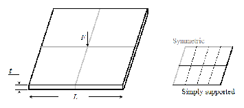
6.1 Simply supported square plate with concentrated load

In this test, a simply supported square plate subjected to a concentrated load at the centre is simulated as shown in Fig. 6. Poisson’s coefficient value is assigned in this example to make the plate incompressible and check for the occurrence of vol- umetric locking. The length of the plate is L=10 and the thick- ness is I=0.2. The material properties are given as I=3.0x106 and v=0.3. The concentrated force F=400. One quarter of the plate is discretised with 4x4 regular mesh by taking advantage of the symmetry of the plate and applying the symmetric boundary condition available in Abaqus. Table 1 lists the ver- tical displacement of the centre point for various elements comparing to the analytical results. The result is compared with a series solution based on Kirchhoff’s theory, considering it to be a thin plate. The displacement at the centre of the plate is given by:

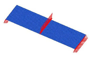
Fig. 7. Clamped strip

The results are given in Table 1.

7 RESULTS

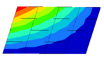
Fig. 8 shows the displacement contours for the simply sup- ported plate, while Fig. 9 shows the results for the clamped strip. Table 1 gives the results of displacements obtained in the numerical tests using the analytical equations, Abaqus S4 gen- eral shell elements, and the nodally integrated new formula-

4P ∞ ∞ sin2 �mπ
sin2 �nπ
𝛿 =
π4 DL6
� � 2 �

(m2 + n2 )2

m=1 n=1

2 �S(29)

Etion for plates. R

Fig. 6. Simply supported square plate with concentrated load

6.2 Clamped strip

In this example, the dimensions of the plate were 220mm x
70mm and its thickness was 3mm. The Young’s modulus was
1195. The load applied at the centre was 100N. The strip is
shown in Fig. 7. Considering the strip to be a beam, the analyt-
ical solution of the displacement at the centre is given by:

Fig. 8. Contour plot of one quarter of simply supported plate

𝛿 =

𝑃𝐿3
192𝐸𝐸
(30)

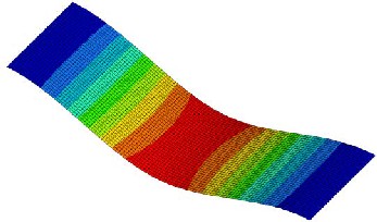
Fig. 9. Contour plot of clamped strip

The research paper published by IJSER journal is about Nodally Integrated Finite Element Formulation for Mindlin-Reissner Plates 1982

ISSN 2229-5518

TABLE 1

DISPLACEMENT RESULTS OF NUMERICAL CASES

Based On Mindlin/Reissner Plate Theory And A Mixed Interpola- tion”, International Journal For Numerical Methods in Engineering, Vol- ume 21, (1985) pp. 367-383.

[9] Abaqus User Subroutines Reference Manual, ver 6.10.

[10] R.D. Cook, D.S. Malkus, M.E. Plesha, and R.J. Witt, Concepts and Ap-

plications of Finite Element Analysis, John Wiley and Sons, 2003. [11] Abaqus Analysis User’s Manual, ver 6.10.

8 CONCLUSION

A new nodally integrated element formulation was described. This formulation makes use of the weighted residual method to derive the assumed strain relations. The nodal integration was performed by averaging over the nodal patch. It was found that Abaqus UELs are not suitable for implementing element formulations where the properties of more than one element are needed at a time for calculation. A new element formulation for four-node quadrilateral elements was imple- mented in Abaqus, and two examples were used to test its behaviour. However, the simulated results have a limited cor- relation with the analytical results, and cannot match the per- formance of the inbuilt elements, as seen in Table 1. This could be attributed to the assumptions made in order to implement in Abaqus UEL, and due to the research being at an initial stage. Improvements in the accuracy of the formulation and in the implementation in Abaqus will help to improve the re- sults.

ACKNOWLEDGMENT

The authors would like to thank the automotive supplier Faurecia for permitting the use of their resources in order to run some of the simulations.

REFERENCES

[1] S. Wolff, “Nodally Integrated Finite Elements”, 18th International Conference on the Application of Computer Science and Mathematics in Architecture and Civil Engineering, K. Gurlebeck and C. Konke (eds.), Weimar, Germany, 07–09 July 2009.

[2] W. Quak, A.H. van den Boogaard, D. González, and E. Cueto, “A

Comparative Study On The Performance Of Meshless Approxima-

tions And Their Integration”, Computational Mechanics, 48, no. 2 (2011) pp. 121-137.

[3] D. Wang, and J. Chen, “Locking-Free Stabilized Conforming Nodal Integration For Meshfree Mindlin–Reissner Plate Formulation”, Com- puter Methods in Applied Mechanics and Engineering, 193.12 (2004) pp.

1065-1083.

[4] G. Castellazzi, and P. Krysl, “Displacement-Based Finite Elements

With Nodal Integration For Reissner–Mindlin Plates”, International

Journal For Numerical Methods In Engineering, 80.2 (2009) pp. 135-162.

[5] G. Castellazzi, and P. Krysl, “A Nine-Node Displacement-Based Finite Element for Reissner–Mindlin Plates Based on an Improved Formulation of the NIPE Approach”, Finite Elements in Analysis and Design, 58 (2012) pp. 31-43.

[6] E. Giner, N. Sukumar, J.E. Tarancon, and F.J. Fuenmayor, “An

Abaqus Implementation Of The Extended Finite Element Method”,

Engineering Fracture Mechanics, 76, no. 3 (2009) pp. 347-368.

[7] K. Park, and G.H. Paulino, “Computational Implementation Of The PPR Potential-Based Cohesive Model In ABAQUS: Educational Per- spective”, Engineering Fracture Mechanics (2012).

[8] K.J. Bathe, E.N. Dvorkin, “A Four-Node Plate Bending Element