International Journal of Scientific & Engineering Research, Volume 6, Issue 4, April-2015 8
ISSN 2229-5518
Modeling soil profile using GIS and Geo- statistical algorithms
Eng. Mohammed Abd El Fadil Ismail, Prof. Dr. Ali Abd El Fatah, Dr. Ashraf M. Hefny
————————— ——————————
y the early beginning of the current century the geotechnical scientists started trying the application
of both GIS and geo-statistics in their various
applications. One of these applications was the soil
characterization specially for those mixed soils with
anomalies and traces which is difficult to be characterized
by only simple system of boreholes and may need some test like Cone penetration test (CPT) that gives a continuous representation of the soil profile. Geo- statistics in several studies has proved that it could give acceptable results in 3D soil profiling. The implementation of Geo-statistics for this purpose needs to have in mind some consideration like:
• The needed software to be used considering its capabilities in both data and outputs manipulation and representation from one side and its Geo- statistical capabilities from another side.
• The problems that may rise in case the data is from different sources or it is distributed on a large area of study.
• The suitable geo-statistical algorithm to be applied for the modeling process
In 1950's Georges Matheron recognized the approaches of the geologist D.G Krige in spatially correlating large amount of data in predicting a real gold concentrations in South Africa. In 1965, in the Ecole des Mines, France Matheron was able to formulate the equations and algorithms of what is currently known as Geo-statistics and he honors the role of D.G krige by using the term "Kriging" to describe the process of estimating the values at un-sampled locations. [R1]
Geo-statistics could be defined as “Statistical technique offers a way of describing the spatial continuity of natural phenomena and provides adaptations of classical regression techniques to take advantage of this continuity.” [R2] It depends on Topler first law of geography "Things that are closer together tends to be more alike than things that are far apart". It assumes that all values in the study area are the result of a random process with dependence. In a spatial or temporal context, such dependence is called autocorrelation. This concept was abstracted through an equation:
Z(s) = µ(s) + ε(s)+ m [R3] (1)
where Z(s) is the phenomena to be predicted at location s
and µ is a mean (structural function describing the
structural component) which is known or unknown and it is either constant or varies with location in data with trends, and these properties depends on the type of the used Kriging. ε(s)is the stochastic but spatially auto- correlated residuals from µ(s) (i.e. the regionalized variable [R4]) and m is a constant account for un-biasness and can be defined as a random noise having a normal distribution with a mean of 0 and a variance σ2. [R5]
Based on the above three main tasks are needed to perform geo-statistical modeling. First, is the determination of µ(s)or trends in data and to make data
de-trending through transformation techniques. This to account for the assumption of Geo-statistics is a random process with dependence. Second, the de-trended data is used twice: to uncover the dependency rules (estimate the spatial autocorrelation or get a function for the regionalized variable) and to make predictions using generalized linear regression techniques (kriging) of unknown values. The constant in this linear regression is a matrix calculated based on the spatial autocorrelation calculated for the sample points of known data. The spatial autocorrelation could be represented by the semi- variogram [R5]
IJSER © 2015 http://www.ijser.org
International Journal of Scientific & Engineering Research, Volume 6, Issue 4, April-2015 9
ISSN 2229-5518
The semi-variance can be estimated from the sample data using the formula:
1 n 2
![]()
γˆ( h ) = ∑ z( s ) − z( s+h )
2 n i=1
(2)
Sgems can be defined as an open-source computer
software package for 3D geo-statistical modeling [R8]. It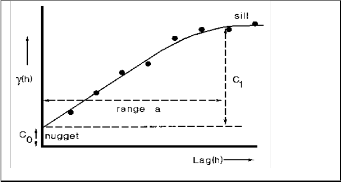
where n is the number of pairs of sample points separated by distance h. The semi-variance can be calculated for different values of h, and s is an indicator for location. A plot of the calculated semi-variance values against h is referred to as an experimental variogram.
Fig1: Variogram
The dependence on the variogram to account for the regionalized variable depends on the consideration of intrinsic Stationarity concept. For semi-variograms, intrinsic stationarity is the assumption that the variance of the difference is the same between any two points that are at the same distance and direction apart no matter which two points are chosen. [R3]
In geo-statistics there are two basic forms of prediction
exist: estimation and simulation. In estimation, a single,
statistically “best” estimate of the spatial occurrence is produced. The estimation is based on both the sample data and on the variogram model. On the other hand, in simulation, many estimate scenarios (sometimes called “images”) of the property distribution are produced, using the same model of spatial correlation as required for kriging. Differences between the alternative maps provide a measure of quantifying the uncertainty, an option not available with kriging estimation. [R6]
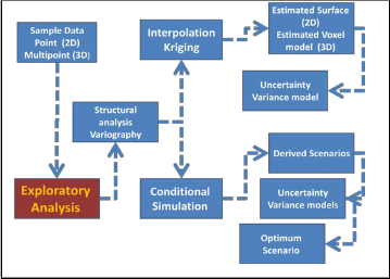
Fig 2. shows the geo-statistical modeling process for both
estimation and simulation
implements many of the classical geo-statistics algorithms, as well as new developments made at the SCRF (Stanford center for reservoir forecasting) lab, Stanford University. Sgems relies on the Geo-statistics Template Library (GsTL) to implement its geo-statistical routines, including: Kriging, Multi-variate kriging (co- kriging), Sequential Gaussian simulation, Sequential indicator simulation, Multi-variate sequential Gaussian and indicator simulation and Multiple-point statistics simulation. The main features of Sgems are: Comprehensive geo-statistical toolbox, Standard data analysis tools: histogram, QQ-plots, variograms,..., interactive 3D visualization, Scripting capabilities: Sgems embeds the Python scripting language, that allows to automatically perform several (repetitive) actions, Use of plug-ins to add new geo-statistics algorithms, support new file formats, or increase the set of script commands. [R8].Sgems has two main types of geometric objects for data representation and inputs in the modeling process. These inputs could be either pointset (like the case of boreholes that are represented as 3D points carrying in their attributes the properties needed to be modeled), or grids that are considered as an output also. These grids could be either Cartesian ordinary grids or masked grids to show a certain geologic element considering that the term grid is used to represent also the 3D voxel model not like ArcGIS used to represent 2D cellular model only. These grids could be also geographical referenced (Geo- referenced) by entering real coordinates for their origin. Whatever the type of this object, it could be stored in either Ascii files in Geo-EAS [10] format used by GSLIB [9] or native Sgems binary files. 1
As a GIS product ArcGIS can deal with both raster and vector data, so it can be used not only in representing the boreholes point set or interpolated grids as Sgems but it can give a complete representation for the whole working site elements that could be needed for the modeling process. But still ArcGIS is missing the capability of dealing with real 3D Voxel data and this is one of the reasons of not using its Geo-statistical module in the modeling process in the practical part of the research. This deficit in ArcGIS was covered in some ArcGIS third party applications (ArcGIS extensions) like Target of Geosoft Co., ArcHydro subsurface analyst of Aquaveo Co., EnterVol of Ctech and Rockworks of Rockware Co., [R11] but still some of these extensions do not support Geo-statistical algorithms like Rockworks or they are like EnterVol not supporting all the geo-statistical algorithms needed for different types of data. For the main Geo- statistical extension of ArcGIS, it can deal only with 2D and not supporting the categorical data simulation![]()
Fig .2. Geo-statistical modeling process
1
GSLIB is an acronym for Geo-statistical software library. This name
was used for a collection of geo-statistical programs and libraries developed in Stanford university. [13]
IJSER © 2015 http://www.ijser.org
International Journal of Scientific & Engineering Research, Volume 6, Issue 4, April-2015 10
ISSN 2229-5518
algorithm which is the most suitable for boreholes modeling.
There are three means of integration between ArcGIS and
Sgems for soil profile modeling: [R12]
• Manual/Semi-automated integration depending on
GSLIB Ascii files and Param XML Ascii files
• Call a program (like ArcGIS) from Sgems through Python and C++ plug-in and use Sgems interface as the main working interface
• Call Sgems externally from another program (e.g.
ArcGIS) and let Sgems work from behind as if it is a service not an application (Through Python scripts)
In the case study the first integration technique was adopted. It depends on the nature of the GSLIB and Param files and the ability to create and edit them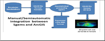
through delimited text editors like notepad or Excel. The process of integration starts by the conversion of the source borehole data to Ascii file with the GSLIB format. This conversion depends on the package incubating the source data which in this case it was ArcGIS software. This conversion could be done manually through some tools in ArcGIS in addition to delimited text editor like Excel or it could be done automatically through a programming with a language that depends on the package carrying the source data which in the case of ArcGIS Python or .net or any other com compliant language. After this conversion the GSLIB file become readable to the Sgems and it could be read as grid or pointset (which is the one used in the case of boreholes). The file is then used in interpolation process (Estimation or simulation). The parameters file of the interpolation process could be also produced using the text editor but mainly it is generated through the Sgems interface due to the fact of needing manual intervention and evaluation in the determination of variograms parameters. The final output grid (as a result of interpolation and post processing) can be saved as GSLIB file and can be manipulated to be read by ArcGIS. This manipulation could be manually through ArcGIS tools and text editor or could be through a program. Finally this manipulated file can be present as 3D points in ArcGIS. It is worth considering that the process discussed in this section is not considering the ArcGIS 3D party programs mentioned above which enables ArcGIS to represent data in 3D voxel representation.
Fig 3. Manual interaction between Sgems and ArcGIS
In dealing with categorical data like soil categories a type of kriging called indicatior kriging is always used. Indicator Kriging (IK) uses the basic kriging paradigm
but in the context of an indicator variable. Indicator kriging based on modeling the uncertainty about a category sk, k=1.....N of the categorical variable s at the un-sampled location u. The uncertainty is modeled by the conditional probability distribution function of the discrete random variable S(u):
p(u: sk |(n)) = p{S(u) = sk|(n)} (3)
where the conditioning information consists of n
neighborhood categorical data s(uα ). Each conditional
probability p(u;sk|(n)) is also the conditional expectation
of the class-indicator random variable I(u;sk):
p(u;sk|(n)) = E{I(u;sk)|(n)} (4)
The kriging estimator for the indicator random variable is
defined as
[I(u;sk] - E{I(u;sk)] (5)
= ∑n(u) λ (u; s )[I(u ; s ) − E{I(u ; s )}]
where λα(u; sk ) is the weight assigned to the indicator
datum I(uα; sk ) interpreted as a realization of the
indicator random variable I(uα ; sk ) [R14]
Effectively indicator kriging produces a conditional
probability distribution for each category at each grid location in the study region. From this probability distribution a category needs to be derived and so there must be a post-processing classification algorithm applied to the output of IK. There are a number of different post- processing classification algorithms, such as maximum likelihood. These algorithms tend to over represent the category (litho-type) with the greatest global proportion and under represent or ignore the category of least global proportion [R15]
While to simulate categorical data sequential indicator is used to simulate the spatial distribution of the mutually exclusive categories (litho-types) sk conditional to the data set {s(uα) ,α =1........,n} . A simplified work flow of the procedure, [R15] is as follows:
1. Define a random path visiting each node of the
study area grid only once.
2. At each node u′:
a. Use ordinary indicator kriging to determine the conditional probability of occurrence of each category sk ,[p(u′ ;sk | (n))]. The (n) conditioning information consists of the neighborhood original indicator data and previously simulated indicator values.
b. Build a cumulative distribution function-
type function by adding the corresponding probabilities of occurrence of the categories
c. Draw a random number p uniformly distributed in [0,1]. The simulated category
at location u′ is the one corresponding to the probability interval that includes p.
d. Add the simulated value to the conditioning data set.
3. Proceed to the next node along the random path and repeat steps (a) to (d).
4. Repeat the entire sequential procedure with a
different random path to generate another realization
IJSER © 2015 http://www.ijser.org
International Journal of Scientific & Engineering Research, Volume 6, Issue 4, April-2015 11
ISSN 2229-5518
Two case studies were applied using this integration technique.
• The first one was on 30 CPT logs taken from a costal project in Kuwait.
• The second one was on 850 boreholes covering 10th of Ramadan city in Sharkia governorate in Egypt.
As mentioned, the city scale modeling of data could generate a number of problems considering the fact the data will be from different sources. Hence, in this context three problems are addressed. First is the samples format whether they are from CPT test or drilling boreholes. Second, is the classification of data to get the categories required for the SIS in case the source is the form of soil reports from different sources. Third, is the assumption of autocorrelation and how it could be fulfilled on the large city scale considering the software limitations. The following lines shows how these problems were handled in the case study
In order to convert the CPT log data to soil classes, the soil behavior type charts (SBT) are used like Robertson
1986, Robertson 1990, Olsen and others. [R16] The problem comes in the correlation between both the continuous line of the cone resistance (qc) charts and the friction factor (Rf) to produce points to be represented on a SBT. This requires the superposition between the two charts to account for the local variations in each chart to get influencing points that need to be considered in the projection on the SBT. Another problem is the dense and small local variations that needs to be generalized. Hence, the following steps were followed to overcome these problems.
First: the PDF files of the CPT logs were entered as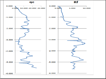
images to ARCGIS software and digitized to get a vector representation for both the Rf and qc charts. For those clear charts, the ArcScan extension was used for automatic digitizing while for others they were digitized manually considering the raster snapping capabilities of ARCGIS
Fig 4. Cone resistance and friction factor curves
Second: The lines of the two charts qc and Rf were smoothed to minimize the local variations with a suitable degree using the Generalize tool of ArcGIS that uses Douglas-Peucker [R17] simplification algorithm with a suitable tolerance.
Third: a superposition between the two generalized
charts was done using a developed program that
recognized the inflection vertices in each chart and
getting the corresponding value from the second chart
Fourth: these points are projected on the SBT chart to get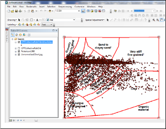
the soil type for each of them. By finishing this step the categories required for SIS are ready for modeling
Fig 5. Robertson points on ArcGIS
Fifth: these points are given the X, Y coordinates of the CPT log and the depth of the point and they were represented as 3D pointset in ArcGIS and converted to the GSLIB format and interpolated using Sgems SIS algorithm.
The second problem considered in the case study was the in consistency of the borehole reports provided from different sources (consultancy offices) in different dates. In the case of 10th of Ramadan city in Egypt, there were more than 800 borehole reports from more than 10 offices, each was following a different methodology is naming the classified soil layers. Average 4 points are recorded for each borehole, then we have more than 3200 record need to be classified in order to create the soil categories required to apply SIS. Moreover this step would be repeated in case there is any change in the categories. Besides that, if we have data from boreholes and others from CPT and it is needed to consider both to refine the SIS Geo-statistical model, it is impossible to use the data with the naming like that mentioned in the table below . Another problem was that all the reports were in Arabic and they were not following any of the standardized systems for soil classification.
IJSER © 2015 http://www.ijser.org
International Journal of Scientific & Engineering Research, Volume 6, Issue 4, April-2015 12
ISSN 2229-5518
4 required | considered (based on Robertson 1986) | |
ﻲﻧﺑ ﺓﺭﺎﺟﺣﻟﺍ ﺭﺳﻛﺑ ﻁﻭﻠﺧﻣ ﻲﻠﻣﺭ ﻁﻟﺯ ﺏﻠﺻ ﺭﺟﺣﺗﻣ ﺭﻣﺣﻣ | 1 | 10 |
ﻑﻳﻌﺿ ﻰﻟﺍ ﺏﻠﺻ ﺭﺟﺣﺗﻣ ﻲﻠﻣﺭ ﻁﻟﺯ ﺭﻣﺣﺃ ﻰﻟﺍ ﻲﻧﺑ ﺔﺑﻼﺻﻟﺍ | 2 | 10 |
ﺢﺗﺎﻓ ﻲﻧﺑ ﻁﺳﻭﺗﻣ ﻰﻟﺍ ﻊﻓﺭ ﻲﻠﻣﺭ ﻁﻟﺯ | 2 | 10 |
ﺢﺗﺎﻓ ﻲﻧﺑ ﻰﻟﺍ ﺭﻣﺣﻣ ﻲﻧﺑ ﻲﻠﻣﺭ ﻁﻟﺯ ﺔﺑﻼﺻﻟﺍ ﻑﻳﻌﺿ ﺭﺟﺣﺗﻣ | 2 | 10 |
ﻕﻣﺎﻏ ﻲﻧﺑ ﻡﻋﺎﻧ ﻰﻟﺍ ﻁﺳﻭﺗﻣ ﻲﻁﻟﺯ ﻝﻣﺭ ﺍﺩﺟ ﺏﻠﺻ ﺭﺟﺣﺗﻣ ﺢﺗﺎﻓ ﻲﻧﺑ ﻰﻟﺍ | 3 | 9 |
ﺭﺳﻛﺑ ﻁﻭﻠﺧﻣ ﺝﺭﺩﺗﻣ ﻲﻁﻟﺯ ﻝﻣﺭ ﺢﺗﺎﻓ ﻲﻧﺑ ﺓﺭﻳﺑﻛﻟﺍ ﺓﺭﺎﺟﺣﻟﺍ | 3 | 9 |
ﺭﺟﺣﺗﻣ ﺭﻣﺣﺃ ﻁﺳﻭﺗﻣ ﻰﻟﺍ ﻥﺷﺧ ﻝﻣﺭ ﺍﺩﺟ ﺏﻠﺻ | 4 | 9 |
ﺭﻣﺣﻣ ﻲﻧﺑ ﻁﺳﻭﺗﻣ ﻰﻟﺍ ﺵﺭﺣ ﻝﻣﺭ ﺔﻳﺭﻳﺟ ﺩﺍﻭﻣ ﻭ ﻲﻣﻁ ﺭﺎﺛﺍ ﻭ ﻊﻳﻓﺭ ﻁﻟﺯﻭ | 4 | 9 |
Hence a method of patterning this data was developed. The results of patterning depends on a preset number of classes (soil categories) or based on the comparison with another fixed pattern like in the case of SBT classes.
The method depends on building what is called
Knowledge tables of the known elements and adding as
much expected names as possible. Sample of the
considered tables:
• Main soil Table: it contains the names of the following for example "ﻞﻣﺭ ، ،ﻂﻟﺯ"
• Complementary soil "ﻲﻠﻣﺭ ، ﻲﻄﻟﺯ"
• Main soil stiffness
• Secondary soil: for mixed soils
• Third soil: for mixed soils
• Texture table: "ﻢﻋﺎﻧ ،ﻦﺸﺧ"
• Connection text table: "ﻰﻟﺍ"
• Main color
• Secondary color
Each value in the main knowledge tables was given a code. Three modules are used for patterns detection developed:
words of each statement and compare them with the texts
in the knowledge tables. For texts that will not match, the
software give the user three choices, either to modify the text and this for those texts with spelling mistakes like "ﻊﻓﺭ " in the previous table and it is originally "ﻊﻴﻓﺭ", or to delete the text, or to add the text to one of the knowledge tables and a code is generated automatically for this new text. This module is run consecutively until all the text match. By the end of this of model all the texts should be coded.
descriptive texts. Each table is given an order based on its consideration in the classification process.
soils recognized in the input data. If the number of required classes is more than the number of main soils, the program starts considering the other parts of the pattern based on their knowledge table order. It is starts
considering the other values based on their frequency in data. In some cases, it may be required by the user to consider both the main soil and the complementary soil as if they are one unit. This is very important when the mix of the main and complementary soils has the dominance in the number of frequent points
This problem comes from the fact that all samples for each soil category in the area of study could be represented in Sgems only by one variogram and this could violate the main concept of Geo-Statistics which is autocorrelation in case of wide areas like in the city scale. This problem was not considered in the case studies in this paper because the data in the areas of study was varying gently and the soil layers were continuous. But in general this problem needs to be considered in such scale of soil profile modeling. It could be simply implemented through the following steps using ArcGIS tools:
1. Apply the Grouping Analysis tool in the spatial
statistics data set to the points of each soil category.
This tool implements a number of grouping
algorithms on of which is the K-nearest [R18]
2. Create the theissen polygons for all the points and
merge the polygons of the points within the same
group in order to cover the whole area of study.
3. Repeat the same two steps for all other soil
categories
4. Union the polygon layers result from step3 to get all
the possible combinations of soil zones
5. Finally, the spatial analyst extension tools of ArcGIS
could be used to eliminate small produced regions
and merge them in neighboring regions to get the final set of interpolation zones.
L.Zane etal 2013 [R19] mentioned a technique to utilize Geo-statistics variogram in determining the seeds required for the grouping and to determine the number
of possible zones based on the range of the variogram. This technique could be used to refine the grouping process
After preparing the categories and the zones using ArcGIS , the SIS was applied on the resulting points in Sgems creating a variogram for each category in each Zone and the output volumetric soil models for the zones were merged using ARCGIS after being converted to 3D points in ArcGIS ArcScene.
IJSER © 2015 http://www.ijser.org
International Journal of Scientific & Engineering Research, Volume 6, Issue 4, April-2015 13
ISSN 2229-5518
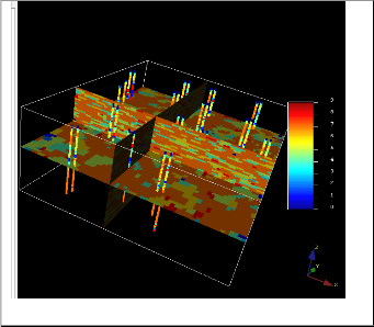
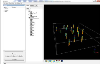
Fig 6. Logs represented as pointsets in Sgems software.
![]()
Fig 7. Interpolated 3D model after applying SIS for one Zone and filtering to remove outliers
The implementation of Geo-statistics in geotechnical modeling is still in its beginning and needs more researches considering all the software that implements these algorithms. The integration between both ARCGIS and Sgems software has showed success in the 3D volumetric modeling of soil profile but still the issue need to be studied more specially for models on city scale. Some of the problems that were faced in modeling on such scale are addressed in this study, but not all of them were tested due to the gently varying nature of data. The mentioned algorithms either for borehole patterning or soil zoning may need to be tested more. For the pattering algorithm, it might to be tested on other versions of English soil reports while for this of Zoning the technique of L.Zane etal 2013 needs to be considered. ArcGIS as a software and it geo-processing showed great capabilities in data preparation, processing, presentation and reporting but still it is missing the suitable tools needed to deal with 3D voxel data and the suitable tools for categorical data simulation, these points which were covered by the Sgems software. A manual integration technique between the two software was presented but still it is needed to develop an automated process for such integration considering the support of both of them for python language
[1] Cressie, N. A. C., "The Origins of Kriging, Mathematical
Geology", v. 22, pp 239–252, 1990
[2] E.H. Isaaks and R.M. Srivastava, "An Introduction to Applied
Geostatistics", Oxford University Press, 1989.
[3] Kevin Johnston, Jay M. Ver Hoef, Konstantin Krivoruchko, and Neil Lucas, ESRI, ArcGIS® 9, "Using ArcGIS® Geostatistical Analyst", Copyright © 2001, 2003
[4] GEORGES MATHERON, "THE THEORY OF REGIONALIZED VARIABLES AND ITS APPLICATIONS", ÉCOLE NATIONAL SUPÉRIEURE DES MINES,
1971.
[5] http://resources.arcgis.com/en/help/main/10.1/index.html
[6] Zhang, Ye.," Introduction to Geostatistics | Course Notes", Dept. of Geology & Geophysics, University of Wyoming, 2011
[7] Nicolas Remy, "Geostatistical Earth Modeling Software: User’s
Manual", 2004
[8] http://sgems.sourceforge.net/
[9] HTTP://WWW.GSLIB.COM/GSLIB_HELP/FORMAT.HTML
[10] TIMOTHY C. COBURN, JEFFREY M. YARUS, R. L. CHAMBERS, "STOCHASTIC MODELING AND GEOSTATISTICS: PRINCIPLES, METHODS, AND CASE STUDIES", VOL. II, AAPG COMPUTER APPLICATIONS IN GEOLOGY 5, 2005
[11] WILLY LYNCH , "3D GIS IN MINING AND EXPLORATION", TECHNOLOGY TRENDS, ESRI ENERGY AND MINING INDUSTRY TEAM, 2013
[12] GUPTA R., "NEW FEATURES IN SGEMS", STANFORD CENTER FOR
RESERVOIR FORECASTING, ANNUAL MEETING, 2010 [13] HTTP://WWW.STATIOS.COM/, 2009
[14] Robin Dunn, "Plurigaussian Simulation of rocktypes using data from a gold mine in Western Australia", EDITH COWAN UNIVERSITY SCHOOL OF ENGINEERING, 2011
[15] Goovaerts, P., Geostatistics for Natural Resources Evaluation.
Oxford University Press, 1997.
[16] ROBERTO QUENTAL COUTINHO, PAUL W. MAYNE, GEOTECHNICAL AND GEOPHYSICAL SITE CHARACTERIZATION 4, CRC PRESS, 2012
[17] DAVID DOUGLAS & THOMAS PEUCKER, "ALGORITHMS FOR THE REDUCTION OF THE NUMBER OF POINTS REQUIRED TO REPRESENT A DIGITIZED LINE OR ITS CARICATURE", THE CANADIAN CARTOGRAPHER 10, 1973
[18] HTTP://RESOURCES.ARCGIS.COM/EN/HELP/MAIN/10.1/INDEX.HT
ML
[19] L.ZANE, B. TISSEYRE, S. GUILLAUME AND B. CHARNOMORDIC, "WITHIN FIELD ZONING USING REGION GROWING ALGORITHUM GUIDED BY GEOSTATISTICAL ANALYSIS", PRECISION AGRICULTURE
2013, WAGENINGEN ACADEMIC PUBLISHERS, SPRINGER, PP. 313-
319, 2013
IJSER © 2015 http://www.ijser.org