International Journal of Scientific & Engineering Research, Volume 4, Issue 4, April-2013 1257

ISSN 2229-5518

Mobility Traces for User Accuracy in Mobile

Network

AMSAVENI.M, MALATHY.S, SATHYAPRIYA.R

Abstract- Location Prediction has attracted a significant amount of research effort. Being able to predict user’s movement would benefit a wide range of communication systems for better resource allocation. The user location prediction problem can be framed as a classification problem, where for a given input of contextual data of the current visit, try to output the correct next location of the user’s. The method is to estimate the physical location of users from a large trace of mobile devices associating with Base Station (BS) in a wireless network. The Soft Classifier Fusion Technique (SCFT) is used to predict the user’s future location. The collection of models, each to model a set of context information best suited it, and focuses on fusing their outputs to provide accurate predictions of the user’s next location. Contextual information may refer to the user’s location, t i m e , and velocity. Each and every user’s behaviors will be noted by the mobile agent in the terms of prediction algorithm EDT (Effective Decision Tree). In this project EDT is implemented for predicting the user’s next location. Different types o f u s e r s a r e used such as r eg ul ar, an d irregul ar. The f us i on approac h is out p erf or ms t h e s t and ard supervised classification algorithms such as SVM or decision tree.

Index Terms- Effective Decision Tree, Location Management, Mobility Traces, Mobility Management, Soft Classifier Fusion Technique, Users Location Prediction, User Mobility Pattern.

1 INTRODUCTION

——————————  ——————————

Fig.1 shows a basic mobile communication with
low power transmitters and receivers at the BS, the Mobile
Today, mobile communication has become the backbone of the society. Each mobile uses a separate, temporary radio channel to talk to the cell site. The cellular concept employs variable low power levels, which allow cells to be sized according to the subscriber density and demand of a given area. As the population grows, cells can be added to accommodate that growth. Frequencies used in one cell cluster can be reused in other cells. A cell is the basic geographic unit of a cellular system.
From cell to cell the conversations can be handed off to maintain constant phone service as the user moves between cells. The Cells in the BS are transmitting over small geographic areas that are represented as hexagons. Depending on the landscape each cell size are varied. At a Particular range the BS can communicate with mobiles. Radio energy dissipates over distance, so the mobiles must be within the operating range of the BS. The early mobile radio system, the BS communicates with mobiles via a
channel.

Station (MS) and also the Mobile Switching Centre (MSC). The MSC is sometimes also called Mobile Telephone Switching Office (MTSO). The BS decay emits the radio signals. A minimum amount of signal strength is needed in order to be detected by the MS which are the hand held personal units.
The channel is made of two frequencies, one for transmitting to the BS and one to receive information from the BS. The BS is also linked to a power source for the transmission of the radio signals for communication and is connected to a fixed backbone network.

 M.Amsaveni is currently pursuing masters degree program in Communication Systems in RVS college of engineering and technology, Coimbatore, India, E-mail: amsaec04@gmail.com

 S.Malathy is currently working as associate professor in the department of

electronics and communication engineering in RVS college of engineering

and technology, Coimbatore, India, E-mail: joymalaty@gmail.com

 R.Sathyapriya is currently pursuing masters degree program in

Communication Systems in RVS college of engineering and technology, Coimbatore, India, E-mail id: priyramme@gmail.com.

Fig: 1 Basic Cellular Structure

The region over which the signal strength lies above such a threshold value is known as the coverage area of a BS. The fixed backbone network is a wired network that links the BS and also the landline and other telephone networks through wires.
A. Mobility Management (MM)
IJSER © 2013 http://w w w .ijser.org

International Journal of Scientific & Engineering Research, Volume 4, Issue 4, April-2013 1258

ISSN 2229-5518

The major functions of a Global System for Mobile Communication (GSM) are the Mobility Management (MM). The objective of MM is to track the users for allowing mobile phone services to be delivered to them.
The two components of MM are Location
Management and Handoff Management. B. Location Management
The current location of the mobile host is determined by using the location management process.
Two different services are present in the location

alternative path

(e.g home)

Road

(e.g work)

Normal sequence

management. There are mobile tracking and locating. The process of tracking the current location of the mobile host is known as mobile tracking. The process of finding the current location of the mobile host for the delivery of an incoming call is known as mobile locating.
Location updating and paging generate traffic in mobile networks. Traffic need to be reduced by using several attempts. One of the attempts is to predict the future location of the user by using the user movement behaviour and their traffic characteristics. If the user’s future location is known in advance, no location updating is necessary. The user’s overload can be reduced by maintaining the knowledge of the user’s history of movement behaviour.
C. Classification of Users
If the network user is free to move, it is difficult to track because of randomness increase in user movement. Depending on the amount of randomness, user’s are classified in to class A and class B.
Class A: This type of users is highly predictable,
because the user follows the same path every day.
Class B: This type of users is highly random, because they follow different path every day.
D. User Profiles
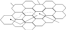
User profiles are used to record the user’s movement behaviours. This user profile allows predicting the user’s behaviours. Several methods are using to estimate the user's movement, location, direction, time and velocity with measuring points.
To create the user profiles developed an efficient, easy and powerful method, which allows a prediction of user's movement on the base of recorded paths. Cell patterns and cell combinations will be stored as user profile along a route between two geographical points. Fig. 2 shows a typical example of an extracted user profile. The same route followed by the user from home to the work every day. Alternatively, another way can also be chosen.

Fig: 2 Example of User Profile

Recording the individual user movement profiles can be done by using GSM measurements. These measurements are used to generate individual user profiles.
For data preparation the user’s id and user’s movement profile are used. This preparation is used to predict the user’s future location. The Mobile id is the unique identifier. Date indicates the movements of displacement are recorded. The period indicates the distinction between the working day and public holiday. The Source Cell indicates the where the user from came. The Destination Cell indicates the where the user is going.

Table. I. Structure of history entry

E. Location Prediction
Numbers of actual locales are referred to as location. The user may move between any of the locations at any point in time. The location history of the user consists of a sequence of location, time and period since the start of observation. The goal of location prediction is to accurately predict lt+1, the next location a user will reside at, given a location history.
F. User Mobility Pattern (UMP)
Mobile users have some regularity in their daily movement, and this regularity can best be characterized by a number of UMP recorded in a profile for each user and indexed by the occurrence time. The UMP is similar to movement patterns but it is more robust in the sense that decreases the UMP sensitivity to small deviations from the User’s Actual Path (UAP).
The number of UMP needed to span the network is greatly reduced, which in turn substantially reduces the time needed for pattern classification. If UMP is described by a cell sequence then model the regular movement of a
mobile user as an edited UMP.
IJSER © 2013 http://w w w .ijser.org

International Journal of Scientific & Engineering Research, Volume 4, Issue 4, April-2013 1259

ISSN 2229-5518

2 LITERATURE SURVEY

(Thuy Van T. Duong and Dinh Que Tran, 2012) proposed the Data mining technique. The 10% outer ratio provides the 0.6 precision and the 20% outer ratio provides the 0.5 precision. The mining algorithms are suitable for mobility prediction in wireless networks. (Sebastien Gambs and Marc Olivier Killijian, 2012) proposed geo privacy mechanisms. This mechanism achieves 75% accuracy for location prediction. (Saikath Bhattacharya and Sudhansu Sekhar Singh, 2011) proposed the movement based model. (Senaka Buthpitiya, et al. 2011) proposed the n gram geo trace modelling. The n gram geo trace method provides
80% accuracy. (Partha Pratim Bhattacharya and Manidipa Bhattacharya, 2011) proposed the prediction based location management scheme. (Said Rutabayirongoga and David erman, 2010) proposed the Markov models and information theoretic techniques. (Teddy Mantoro and Zubaidah Muataz, 2010) proposed the genetic algorithm. The results show that genetic algorithm is efficient in time and number of solutions but the database entries needs more processing to reduce misguided results. (Haitham Abu Ghazaleh,
2010) proposed the Markov Renewal Process (MRP) Model.
The MRP model can be used by network managers for the purpose of efficient network resource management. (Joanna Kolodziej and Samee Ullah Khan, 2009) proposed the Markov model. Markov jump methodology improves the user’s activi ty prediction. (Tamas szalka et al. 2009) proposed the Markovian Mobility Model. (Juha K. Laurila, et al. 2009) proposed the open and dedicated tracks of the Mobile Data Challenge. By using this dedicated task achieves appropriate balance between the necessary privacy protection and simultaneously still maintaining the richness of the data for research purposes. (Dimitrios Katsaros and Yannis Manolopoulos, 2009) proposed the Discrete sequence modelling. (Brian D. Ziebart, et al. 2008) proposed the Probabilistic Reasoning from Observed Context Aware Behaviour (PROCAB) model. This model improvements the compact representation, because of an increased ability to generalize to new situations. (R.V. Mathivaruni and V.Vaidehi, 2008) proposed the mobility prediction technique. This technique achieves 82.6% accuracy, as the motivation for each move is also included. (J. Krumm and E. Horvitz, 2006) proposed the predestinations method. Destination prediction can also be used to detect if a user is deviating from the route to an expected location. (Sang Jun Han and Sung bae, 2006) proposed the novel method. The results were promising enough to confirm that the application works flexibly even in ambiguous situations. (Shiang Chun Liou and Yuehmin
Huang, 2005) proposed the mobility model and a neural
location predictor (NLP) model. The simulation results confirm that NLP can achieve high prediction accuracy. The results are encouraging. (Ian F. Akyildiz, Fellow, and Wenye Wang, 2004) proposed the User Mobility Profile (UMP) framework. This scheme is effective on mobility and resource management by evaluating the blocking, dropping probabilities and location tracking costs in wireless networks. (Rene Mayrhofer, 2004) proposed the architecture for context prediction. (Libo Song, et al. 2004) proposed the Order 2 Markov predictor. Obtain the median accuracy is 72 %. (D. J. Patterson, et al. 2003) proposed the method of learning a Bayesian model. Learned graph model increases the accuracy to 84% of the time on test data, not used for training. (B. P. Vijay kumar and P.Venkataram, 2002) proposed the prediction based location management. The average prediction accuracy was measured and achieved up to 40% to 70% for regular user and 2%to 30% for random movement patterns. (A. Bhattacharya and S. K. Das, 2002) proposed the Adaptive on line algorithm. This algorithm is more efficient for bandwidth management and quality of service provisioning based on reservation.

3 MATERIALS AND METHODOLOGY

3.1 Mobility Prediction

Mobility Prediction (MP) is widely employed in cellular communication. MP can be used to assist handoff management, resource allocation, congestion control and quality of service provisioning at application level it provides the Mobile Location Services. MP is an important to determine the location of the user by carefully manipulating the available information.
The prediction accuracy depends on the user movement model and the prediction algorithm used. Two different techniques are used in the MP. First technique uses the historical movement patterns of the user to predict the user’s where about in future. The second technique predicts the user’s location based on the use of contextual knowledge such as direction and current location. The user’s location determined by based on the mobility behaviour is represented as a set of movement patterns stored in a user profile. Based on the mobility pattern of the user, the EDT algorithm is proposed. The algorithm is used to predict the future location of the user accurately when compared to the existing traditional algorithms.
IJSER © 2013 http://w w w .ijser.org

International Journal of Scientific & Engineering Research, Volume 4, Issue 4, April-2013 1260

ISSN 2229-5518

3.2 Behaviour Based Mobility Prediction

The idea of Behaviour Based Mobility Prediction is to model the regularity mobility patterns based on behaviour factors. Behaviour of users can be characterized in different ways. The characteristic of user’s behaviour are location, time of day and duration. The location factor represents the history of mobility patterns that can be either static or dynamic. Static mobility patterns are fixed structure. Dynamic mobility patterns are caused by drastic changes in operating environmental due to the user mobility.
The time of day indicates that user behaviour changes with function of time. For example the mobility pattern of the student depending on the time of day factor. The student spends the most of the time in school campus in the day time. At evening time he is spend the time in home. The mobility behaviour of the student during the evening will be different from the day time. The duration factor represents the how long the user located in that location. The duration can be classified in to short, medium and long.
The duration factor is based on the user moves in to new location to either moving or stay to perform activities. The mobility behaviour is different to both moving user and stay within the location user.

3.3 Behaviour of User Mobility Model

The Behaviour of regular user mobility model exhibit some regularity in their daily movement and this regularity can be characterized by number of user mobility patterns stored in the profile for each user and indexed by the occurrence time. Consider the family person his daily movement behaviour has s o m e regularity. He s p e n d s the day time in his work place. After 6pm he will reach the home. This is regular movement pattern of family person except week end days. In week end movement behaviour of family person is different from week day behaviour.
The behaviour of irregular user mobility model is the stochastic model with dynamically changing the location. The irregular user mobility model is based on the observation of user movement. It is actually logical function of the user’s speed, direction and position.
Consider the sales man his daily movement behaviour is different from day to day. For example on Monday if he went to Salem, the next day he will going to Madurai. So the mobility pattern is different for irregular user. The irregular user does not follow the same path every day. So predicting the irregular user mobility pattern is difficult accurately when compared to the regular user mobility pattern.

3.4 Proposed Prediction Model

In proposed method SCFT is used to predict the user’s next location. This technique predicts the user’s next location accurately comparatively.
Soft Classifier Fusion Technique (SCFT)
The objective of this project is to predict the next location of a mobile user based on the context, such as the current location and time. To model the user’s mobility patterns and predict the user’s future locations some contributions are used. The contributions are,

 Fusion of model is used for modelling the human

mobility.

 This technique is used for predicting the future significant locations of a user given the user’s current context.

 The fusion model’s location prediction capabilities

with extensive real world data from the MDC
dataset were evaluated.
By fusing the location based model with time based model for next location prediction to achieve the high accuracy level.

lj

lt+l = argmaxlj i i pi ( )

i

This SCFT technique is used to achieve the higher
location prediction Accuracy. SCFT techniques use n models. The SCFT technique used in this project is time based model and the location based model. Each model i can estimate Pi(lj/fi). Where fi is a set of input features of this model (time and current location) and lj represents a possible next location.

The weighting factor is αi. In this technique, weight is

generated in large amount of combinations in order to find the best parameter set for the training data. Use this parameter configuration to perform location prediction based on both training and test data set. The weight combination tries to achieve the highest accuracy. The EDT is used to predict the user’s next location by using
contextual information such as time, location, and velocity,
IJSER © 2013 http://w w w .ijser.org

International Journal of Scientific & Engineering Research, Volume 4, Issue 4, April-2013 1261

ISSN 2229-5518

of different type of users. By comparing EDT concept with existing methods the simulation result shows the effectiveness of this new technique.

3.5 Proposed EDT Algorithm

The proposed prediction algorithm used in this project is EDT algorithm. The EDT is the powerful tool for prediction. EDT is used to predict user location accurately.
The objective of EDT algorithm is to classify correctly as much of the training set as possible. It is helpful to update the training set values easily. In order to predict the next location of regular user, past history (training set) values are used. There are several distinct places are visited by the regular user. These different place IDs are collected to form the training set. However, this approach leads to a user's home and workplace almost always being chosen. The frequent place IDs are selected and applying the SCFT to predict the user’s next location accurately.
Behaviour of mobile users can be characterized in many different ways. Two characteristics are used to define the mobility behaviours. There are location and time of day. The location factor indicates that the movements of mobile users often follow a sequence of locations every day.
For example, in a campus network, lecturers often move to classrooms, laboratories, library, etc whereas departmental staffs often travel around the administrative offices. Therefore, it is possible to predict the next location of a mobile user based on previous location history. The time of day factor identifies the importance of the time when the mobile user moves to the location. The mobility behaviours changes as a function of time.
For example, the movement of lecturers depends on the schedule of classes. That means, lectures will move to the classrooms at the times depending on his own teaching schedule.
Table II Global Training Set
Table II shows the global training set of regular user. Consider the lecture as regular user. Morning 6.50 the lecture is at home which is represented by 1. The lecture reached the college campus canteen by 11.25 which are represented by 7. Staff room location is being represented by 2 and Class room location represented by 4.
The regular user (lecturer) frequently visited the locations are home, class room, canteen and staff room. So the frequent place IDs are collected from the registers and applying the SCFT technique to predict the users next
location. The frequent places ID are shown in the Table III.

Table II Global Training Set

Table III Frequent Place ID

IJSER © 2013 http://w w w .ijser.org

International Journal of Scientific & Engineering Research, Volume 4, Issue 4, April-2013 1262

ISSN 2229-5518

Table IV shows the comparison table which contains the frequent place ID, current location, weighting factor and next location. Based on this frequent place ID and current location, update the weighting factor and predict the user’s next location.

Table V

For irregular user prediction, random motion mechanism technique is applied. This technique will trace the user next location based on the user present location. The mobile agents are used to monitor the user behaviour such as direction, location and distance. Based on this behaviours irregular user next location will be predicted.
For irregular user prediction consider all the directions (North, South, East and West) and distance from the BS. The user moving towards the north direction means that user connected with north side BS. The user moving towards (E, S) means that user connected with nearest BS.

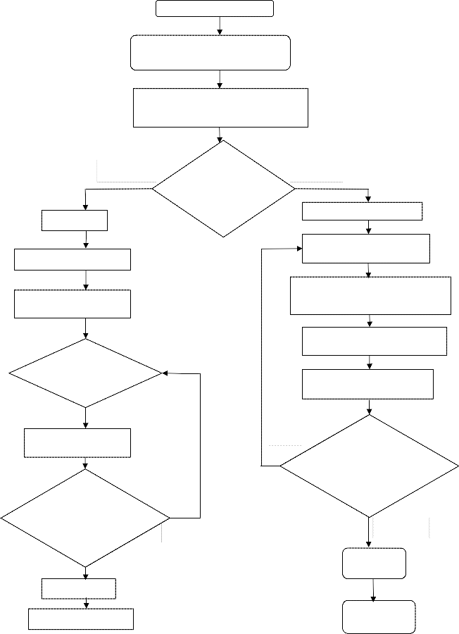
The EDT algorithm procedure is shown in Fig.3
This algorithm performs several steps to predict the user’s next location. The first step of algorithm is analysing the users in an environment. The second step of algorithm is collecting the one month data set (number of visited time, location, and time) for users from Home Location Register (HLR) and Visitor Location Register (VLR). Then identifying the Regular and Irregular user based on the number of visited time in the location registers. Check how many times the user visited the location. If the user visited the location maximum of ten times then the user considered as Irregular User. Otherwise the user is considered as
Regular user.
If the user is regular user means collects the past history (frequent place Ids, number of visited time, duration and time) of the user from the Location Registers. Then identify the frequent places visited by the user. Then compare the past history data with current location data. After comparing the values SCFT technique is applied for accurately predicting the user’s next location. In SCFT technique the weighting factor is updated depending up on the threshold value. This threshold value of 70% is set based on the [23] existing system. In this SCFT technique weighting factor is updated until predicting the user’s next location accurately.
If the accuracy level met the threshold value means that the user next location is predicted and the optimal solution is obtained. If accuracy level is not met the threshold level value means that the weighting factor (αi) value is updated until reaches the optimal solution. Once the optimal solution is reached means the user’s next location can be predicted accurately.
If the user is irregular user means random motion mechanism technique is applied to predict the user’s next location. In random motion technique, the user’s behaviour is monitored by using the mobile agent, and tracing the user’s next location based on the user’s present location. This technique does not use the historical data of the user to predict the user’s next location.
The mobile agent monitors the user’s behaviour
such as velocity and distance from the base station. Depending on these behaviours, the random motion technique predicts the user’s next location. The threshold value of the irregular user used in this project is 30%. This threshold value is set, based on the existing system [23]. After setting the threshold value compares the monitored value and the threshold value.
If the monitored value is greater than the threshold
value means optimal solution is obtained and predicts the next location of the user. If the monitored value is less than the threshold value means again apply the random motion mechanism.
This algorithm consists of several steps to predict
the user next location. Initially analysis is done to check whether the user is regular user or irregular user. In this project 20 users are used for analysing. In these 20 users, the user 11 and user 15 are experimental users and considered as irregular user. The irregular users 12, 13, 14,
16, 17, 18 and 19 are used for analysing purpose. The random motion technique is used for predicting the user’s next location for irregular user.
IJSER © 2013 http://w w w .ijser.org

International Journal of Scientific & Engineering Research, Volume 4, Issue 4, April-2013 1263

ISSN 2229-5518

Analysing the 20 Users

Collect the one month data set for users from

HLR and VLR

Identifying the Regular and Irregular user based on

number of visited time in the location registers

No

Regular User

Check the users has visited maximum of only 10 times

Yes

Irregular User

Collect the training set

Apply the Random motion

mechanism

Identify the frequent places visited

By using this mechanism monitoring the users behaviour such as direction, distance

Compare past history with current location

Set threshold value 30% with respect to existing system

Compare the monitored value with threshold value

Weight updation using SCFT

No

Is monitored value > Threshold Value and

check the accuracy status

Is predicted value> 70%. Threshold value set 70%

based on existing system

No

Yes

Yes

Optimal

Solution

Optimal Solution

Final Prediction Output

Fig: 3 Flow Chart for EDT Algorithm

IJSER © 2013 http://w w w .ijser.org

Final Prediction output

International Journal of Scientific & Engineering Research, Volume 4, Issue 4, April-2013 1264

ISSN 2229-5518

The experimental regular users are user 1, 3, 4 and
8. The regular users 2, 5, 6, 7, 9 and 10 are used for analysing purpose. After identifying the users, if the users are regular user means collecting the past history of the regular user and identifies the most frequent place IDs from the training set and applying the SCFT technique. This technique updating the weighting factor based on the threshold value. If the accuracy level is met means the user next location predicted and the optimal solution is obtained. If accuracy level is not met the threshold level value means the weighting factor (αi) value is updated until reach the optimal solution. Once the optimal solution is reached means the user’s next location can be predicted accurately.

4 RESULTS AND DISCUSSIONS

4.1 Performance Evaluations

User Location Prediction is necessary for reducing the traffic. The prediction accuracy achieved in this project is 90% for Regular User and 45% for Irregular User. Depending on the historical data and user current location the user accuracy is achieved for Regular user and Irregular user. The performance is determined based on the accuracy level. The performance of this project is better than the existing method.

4.2 Simulation Environment

The environment setting of this simulation is wireless. The dimension of the cell’s X and Y direction is 1000x1000. The range of bandwidth is 2MHz. The setting of threshold value is 70% for regular user and
30% for irregular user.

4.3 Simulation Parameters

The simulation parameters used in this paper are number of users, accuracy, training set and cell deployment model. The number of users is 20, training set is 250 and cell deployment model is circle.

4.4 Simulation Results

In existing method the accuracy level of the user location prediction in Order 2 Markov Predictor is 72% [20], MNN model accuracy level for regular user is 40-70% and irregular user accuracy level is 2-30% [23].Active Based Mobility Prediction using Markov Modelling achieves
82.6% level of accuracy [14]. By comparing these models, the EDT algorithm is predicting the user location accurately.
Fig.4 shows the user graph for regular user and irregular user prediction accuracy. When training set
values are increased the accuracy percentage values are
also increased. The Regular users achieve 90% accuracy and Irregular users achieve 45% accuracy.
For Regular user 50 training set values provide the 10% accuracy level of user’s location prediction. 100 training set values provide the 35% accuracy. 150 training set values provide the 60% accuracy. 200 training set values provide the 80% accuracy and 250 training set values provide the 90% accuracy.
In paper [12] Prediction by Partial Match (PPM)

Scheme is used to predict the user next location. This scheme achieves 25% accuracy for 100 training set. 150 training set achieves 28% accuracy, whereas EDT algorithm achieves 35% accuracy for 100 training set. 150 training set achieves 60% accuracy. This comparison shows, the EDT algorithm performs better than PPM scheme.

Fig: 4 User Graph

The Fig.5 shows the Velocity graph for Regular user. The accuracy value is varied according to the speed of the user movement. The users are travelling in different vehicles such as car, bike and train. Depending on the speed of the vehicle, the user location will be predicted
Depending on the car velocity the user location will be predicted. The prediction a c c u r a c y is high when the user travels by car, because the velocity of the car is easily predictable when compared to the bike and train. The common training set values are used in x axis. The y axis represents the accuracy level. When training set values are increased the accuracy level values also increased.
IJSER © 2013 http://w w w .ijser.org

International Journal of Scientific & Engineering Research, Volume 4, Issue 4, April-2013 1265

ISSN 2229-5518

Fig: 5 Velocity Graph for Regular User

The Regular user travels by bike. Depending on the bike velocity the user location will be predicted. The prediction accuracy is more when the user travels by bike, because the velocity of the bike is slightly easy to predict when compared to the train.
The Regular user travels by train. Depending on the train velocity the user location will be predicted. The prediction of the user location is less while the user travelled by train.
In Car velocity graph regular user achieves 10% accuracy level for 50 training sets. 100 training sets provide 40% accuracy. 150 training sets provide 75% accuracy. 200 training sets provide 85% accuracy and 250 training sets provide 88% accuracy.
In bike velocity graph t h e regular user achieves
5% accuracy level for 50 training sets. 100% training sets provides 35% accuracy. 150 training sets provide 55% accuracy. 200 training sets provide 65% and 250 training sets provides 68% accuracy.
In train velocity graph the regular user achieves
5% accuracy level for 50 training sets. 100% training sets provide 27% accuracy. 150 training sets provide 45% accuracy. 200 training sets provide 55% and 250 training sets provide 58% accuracy.
The car, bike and train speeds are varied normally.
Prediction of location is difficult when the user is travelling by the train because BS signal is not obtained properly. So accuracy of prediction is low. Predicting the user location can be done accurately when the user
travelling by car and bike. Because these type of users obtain the BS range properly.
Fig.6 shows the velocity graph for irregular user. The Irregular user travels by car. Depending on the car velocity the user location will be predicted. The prediction accuracy is high when the user travels by car, because the velocity of the car is easily predictable when compared to the bike and train. The common training set values are used in x axis. The y axis represents the accuracy level. When training set values increases the accuracy level values also increases.
The Irregular user travels by bike. Depending on the bike velocity the user location will be predicted. When the user travels by bike, the prediction accuracy is more, when compared to the train.
The Irregular user travelled by the train. Depending on the train velocity the user location will be predicted. The prediction of the user location is less while the user travelled by train.
The Irregular user travels by car. The velocity of the irregular user achieves 8% accuracy for 50 training sets. 100 training sets provide 28% accuracy. 150 training sets provide 48% accuracy. 200 training sets provide

55% accuracy and 250 training sets provide 58% accuracy.

Fig: 6 Velocity Graph for Irregular User

The Irregular user travels by bike. The velocity of the irregular user achieves 5% accuracy for 50 training sets.
100% training sets provide 23% accuracy. 150 training sets provide 40% accuracy. 200 training sets provide 45% and
250 training sets provide 48% accuracy.
IJSER © 2013 http://w w w .ijser.org

International Journal of Scientific & Engineering Research, Volume 4, Issue 4, April-2013 1266

ISSN 2229-5518

The Irregular user travels by train. The velocity of the irregular user achieves 5% accuracy for 50 training sets.
100% training sets provide 18% accuracy. 150 training sets provide 30% accuracy. 200 training sets provide 33% and
250 training sets provide 35% accuracy.
Fig. 7 shows the comparison graph for different algorithms such as EDT algorithm, Genetic Algorithm (GA) and Neural Network (NN). This graph shows, at particular time how the algorithms works and predict the next location of the users.

Fig: 7 Comparison Graph

The accuracy level of the EDT algorithm at 5ms is
5% accuracy. The accuracy is 25% at 10ms, 60% at 15ms,
80% at 20ms, 88% at 25ms and 90% at 30ms.The accuracy level of the GA algorithm at 5ms is 5% accuracy. The accuracy is 20% at 10ms, 48% at 15ms, 63% at 20ms, 72% at 25ms and 73% at 30ms. The accuracy level of the NN algorithm at 5ms is 5% accuracy. The accuracy is 18% at
10ms, 40% at 15ms, 53% at 20ms, 57% at 25ms and 59% at
30ms.

5 CONCLUSION

In this project SCFT Technique is used for predicting the user’s future location with high accuracy. The performance of the technique has been verified for prediction accuracy by considering different movement pattern of users. Simulation is also carried out for different movement patterns such as regular and irregular to predict the future location of the user. The average prediction
accuracy was measured and achieved up to 90% for
regular users and 45% for irregular users. The proposed method helps in reducing the traffic for location management by predicting the future location of the users.

COMPARISON TABLE VI

TABLE VII

TABLE VIII

IJSER © 2013 http://w w w .ijser.org

International Journal of Scientific & Engineering Research, Volume 4, Issue 4, April-2013 1267

ISSN 2229-5518

REFERENCES

[1]. Thuy Van T. Duong and Dinh Que Tran “An Effective Approach for Mobility Prediction in Wireless Network based on Temporal Weighted Mobility Rule” International Journal of Computer Science and Telecommunications, Volume 3, Issue 2, 2012.
[2]. Sebastien Gambs and Marc-Olivier Killijian, “Next Place Prediction Using Mobility Markov Chains”, MPM’12, April 10, 2012.
[3]. Saikath Bhattacharya and Sudhansu Sekhar Singh,” Location Prediction Using Efficient Radial Basis Neural Network “International Conference on Information and Network Technology, Volume.4, 2011.
[4]. S. Buthpitiya, Y. Zhang, A. Dey, and M. Griss. “n- gram Geotrace Modelling” International Conference, pages 97–114, 2011.
[5]. Partha Pratim Bhattacharya, Manidipa Bhattacharya,” Artificial Neural Network Based Node Location Prediction for Applications in Mobile Communication” International Journal of Computer Applications in Engineering Sciences, Volume 1, Issue 2,
2011.
[6]. Said Rutabayirongoga and David erman,” Predictive Models for Seamless Mobility”, School of Computing/Blekinge Institute of Technology HET NETs, pages 273–284, 2010.
[7]. Teddy Mantoro, and Zubaidah Muataz,” Mobile User Location Prediction: Genetic Algorithm-Based Approach”, IEEE Symposium on Industrial Electronics and Applications, October 3-5, 2010.
[8]. Haitham Abu-Ghazaleh, “Application of Mobility Prediction in Wireless Networks Using Markov Renewal Theory”, IEEE Vehicular Technology, Conference in Singapore, Volume 59, Issue 2, 2010.
[9]. Joanna Kolodziej and Samee Ullah Khan “An Application of Markov Jump Process Model for Activity Based Indoor Mobility Prediction in Wireless Networks” Frontiers of Information Technology (FIT), 2009.

[10]. Tamas Szalka, Sandor Szabo and Peter Fulop, “Markov model based Location prediction in wireless cellular networks” Information communication Journal,

Volume 3, 2009.
[11]. J. K. Laurila, D. Gatica-Perez, I. Aad, J. Blom, O. Bornet, T. Do, O.Dousse, J. Eberle, and M. Miettinen. “The mobile data challenge: Big data for mobile computing research”. In Mobile Data Challenge by Nokia Workshop,
2009.
[12]. Dimitrios Katsaros and Yannis Manolopoulos, “Prediction in Wireless Networks by Markovchains”2009.
[13]. B. D. Ziebart, A. L. Maas, A. K. Dey, and J. A. Bagnell. “Navigate like A Cabbie: probabilistic reasoning from observed context-aware behaviour”. In Ubi Comp, pages 322–331, 2008.
[14]. R.V. Mathivaruni and V.Vaidehi,” An Activity Based Mobility Prediction Strategy Using Markov Modeling for Wireless Networks”, WCECS, October 22
- 24, 2008.
[15]. J. Krumm and E. Horvitz, “Predestination: Inferring destinations from partial Trajectories” In Ubi comp, volume 4206, pages 243– 260, 2006.
[16]. Sang-Jun Han and Sung-Bae Cho, “Predicting User’s Movement with a Combination of Self-Organizing Map and Markov Model” ICANN, Part II, Page No 884 – 893,
2006.
[17]. Shiang-Chun Liou and Yueh-Min Huang,” Trajectory Predictions in Mobile Networks “International Journal of Information Technology Volume.No.11, 2005.
[18]. Ian F. Akyildiz, Fellow, and Wenye Wang, “The Predictive User Mobility Profile Framework for Wireless Multimedia Networks” IEEE/ACM Transactions of Networking,, Volume No 12, Page No
6,2004.
[19]. R. Mayrhofer. “An Architecture for context prediction”. Trauner, 2004.
[20]. Libo Song, David Kotz, Ravi Jain, Xiaoning He” Evaluating location Predictors with extensive Wi-Fi mobility data” IEEE Information Communication, 2004.
[21]. D. J. Patterson, L. Liao, D. Fox, and H. Kautz. Inferring high level behaviour from low-level sensors. In Ubicomp2003, Volume 2864, pages 73–
89, 2003.
IJSER © 2013 http://w w w .ijser.org

International Journal of Scientific & Engineering Research, Volume 4, Issue 4, April-2013 1268

ISSN 2229-5518

[22]. D. Ashbrook and T. Starner. “Using GPS to learn significant locations and prediction movement across multiple users” Personal and Ubiquitous Computing, Page No: 275–286, 2003.
[23]. B. P. Vijay kumar and P. Venkataram, “Prediction- based location Management using multilayer neural networks” Indian Institute of Science, Volume 82, 2002.
[24]. A. Bhattacharya and S. K. Das. “Lezi-update: an information theoretic Frame work for Personal mobility tracking in pcs networks Volume 8, Page No121–135,
2002.
IJSER © 2013 http://w w w .ijser.org