any ϵ > 0, choosing d = [
] ensures that the
International Journal of Scientific & Engineering Research, Volume 3, Issue 10, October-2012 1
ISSN 2229-5518
Mitigation of Capacity Region of Network and Energy Function for a Delay Tolerant Mobile Ad Hoc Network
Dasari Bharati, M.V. Rajesh
Abstract— We investigate two quantities of interest in a delay tolerant mobile ad hoc network: the network capacity region and the minimum energy function. The network capacity region is defined as the set of all input rates that the network can stably sup port considering all possible scheduling and routing algorithms. Given any input rate vector in this region, the minimum energy function establishes the minimum time average power required to support it. In this work, we consider a cell-partitioned model of a delay-tolerant mobile ad hoc network with general Markovian mobility. This simple model incorporates the essential features of locality of wireless transmissions as well as node mobility and enables us to exactly compute the corresponding network capacity and minimum energy function. Further, we propose simple schemes that offer performance guarantees that are arbitrarily close to these bounds at the cost of an increased delay.
Index Terms— Capacity region, Delay tolerant networks, Minimum energy scheduling, Mobile ad-hoc network and Queueing analysis.
—————————— ——————————
WO quantities that characterize the performance limits of a mobile ad hoc network are the network capacity region and the minimum energy function. The network capacity
region is defined as the set of all input rates that the network can stably support considering all possible scheduling and routing algorithms that conform to the given network structure. The minimum energy function is defined as the minimum time average power (summed over all users) required to stably support a given input rate vector in this region. Here, by stability we mean that the input rates are such that for all users, the queues do not grow to infinity and average delays are bounded. In this paper, we exactly compute these quantities for a specific model of a delay- tolerant mobile ad hoc network.
Asymptotic bounds on the capacity of static wireless networks and mobile networks are developed [2], [3]. The work in reference [3] shows that for networks with full uniform mobility, if delay constraints are relaxed, a simple 2-hop relay algorithm can support throughput that does not vanish as the number of network nodes N grows large. Recent work in [4] generalizes this model and investigates capacity scaling with non-uniform node mobility and heterogeneous nodes. Capacity-delay tradeoffs in mobile ad hoc networks are considered in [8] - [12]. Flow-based characterization of the network capacity region is presented in several works (e.g., [7], [13], [14]).
————————————————
However, little work has been done in computing the exact capacity and energy expressions for these networks. Exceptions include a closed form expression for the capacity of a fixed grid network in [5], an expression for the exact information theoretic capacity for a single source multicast setting in a wireless erasure network [6], and an expression for the capacity of a mobile ad hoc network in [8] that uses a cell-partitioned structure. The work [8] quantizes the network geography into a finite number of cells over which users move, and assumes that a single packet can be transmitted between users who are currently in the same cell, while no transmission is possible between users currently in different cells.
In this work, we extend this model to more general scenarios allowing adjacent cell communication and different rate power combinations. Specifically, we extend the simplified cell- partitioned model of [8] (which only allows same cell communication and considers i.i.d. mobility) to treat adjacent cell communication. We establish exact capacity expressions for general Markovian user mobility processes (possibly non- uniform), assuming only a well-defined steady state location distribution for the users. Our analysis shows that, similar to [8], the capacity is only a function of the steady state location distribution of the nodes and a 2-hop relay algorithm is throughput optimal for this extended model as well. Further, our analysis illuminates the optimal decision strategies and precisely defines the throughput optimal control law for choosing between same cell and adjacent cell communication. We then use this insight to design a simple 2-hop relay algorithm that can stabilize the network for all input rates within the network capacity region. We also compute an upper bound on the average delay under this algorithm.
We next compute the exact expression for the minimum
energy required to stabilize this network, for all input rates
within capacity. Our result demonstrates a piecewise linear
structure for the minimum energy function that corresponds to
IJSER © 2012 http://www.ijser.org
International Journal of Scientific & Engineering Research, Volume 3, Issue 10, October-2012 2
ISSN 2229-5518
opportunistically using up successive transmission modes. Then we present a greedy algorithm whose average energy can be pushed arbitrarily close to the minimum energy at the cost of an increased delay.
Before proceeding further, we emphasize that the network
capacity and minimum energy function derived in this paper
are subject to the scheduling and routing constraints of our
model as described in the next section. Specifically, in this
work, we do not consider techniques that “mix” packets, such
as network coding or cooperative communication, which can increase the network capacity and reduce energy costs. In fact,
in Section of “Capacity gaining by network coding”, we present an example scenario that shows how network coding in conjunction with the wireless broadcast advantage can increase the capacity for this model. Calculating the network capacity region and the minimum energy function when these strategies are allowed is an open problem in general in network information theory and is beyond the scope of this paper.
We use a cell-partitioned network model (Fig. 1) having ‘C’ non-overlapping cells (not necessarily of the same size/shape). There are ‘N’ users roaming from cell to cell over the network
according to a mobility process. Each cell c ∈ {1, 2, … . , C} has a
set of adjacent cells ‘B ’ that a user can move into from cell c.
by a finite state ergodic Markov Chain. In particular, let
P = {P } be the transition probability matrix of this Markov
Chain. Then P represents a conditional probability that, user
moves to cell j in the current slot given that it was in cell i in the
last slot. Note that P > 0 only if j is an adjacent cell of i, i.e., j ∈
Bi. It can be shown that the resulting mobility process has a
well-defined steady state location distribution π = {π } over the cells c ∈ {1, 2, … . , C} that satisfies πP = π and is the same for
all users. However, this distribution could be non-uniform over
the cells. We assume that in each slot, users are aware of the set of other users in the same cell and in adjacent cells. However, the transition probabilities associated with the Markov Chain P are not necessarily known.
It can be shown (see, for example, [18]) that the mobility
process discussed above has the following property. Let
χ(t) ∈ {1, 2, … . , C} denote the location of a user in timeslot t. Then, for all integers d > 0, there exist positive constants α, γ such that ∀ ∈ {1, 2, … . , C}, the following holds:
(1 ) [ ( ) = | ( )]
(1 ) (1)
where α > 1 and 0 < γ < 1. Moreover, the decay factor γ is
given by the second largest eigenvalue of the transition
probability matrix P (see [17]). From this, it can be seen that for
( / )
The maximum number of adjacent cells of any cell is bounded![]()
any ϵ > 0, choosing d = [
] ensures that the
( )
by a finite constant J. We define the network user density as
θ = N/C users/cell. For simplicity, ‘N’ is assumed to be even and N ≥ 2. Note that there could be “gaps” in the cell structure
due to infeasible geographic locations. We assume that the gaps
do not partition the network, so that it is possible for a single
user to visit all cells. We assume ‘C’ is the number of valid cells,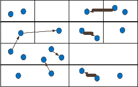
not including such gaps.
R2
R2 R1
R2
R1
R2 R1
Fig. 1. An illustration of the cell-partitioned network with same and adjacent cell communication. Cells that share an edge are assumed to be adjacent.
Time is slotted so that each user remains in its current cell for a timeslot and potentially moves to an adjacent cell at the end of the slot. We assume that, each user i moves independently of the other users according to a mobility process that is described
conditional probability that the user is in cell ‘c’ at time t + d is
within π ϵ of the steady state probability π of being in cell c,
irrespective of the current location. This implies that the
Markov Chain converges to its steady state probability
distribution exponentially fast. Using the independence of user mobility processes, the following can be shown about
functional of the joint user location process χ⃗ (t).
Lemma 1. Let ( ) = ( ( ), … . , ( )) be the vector of current
user locations, where ( ) represents the cell of user i in slot t.
Let �( ( )) be any non-negative function
of ( ), 𝑖. �. , �( ( )) ≥ 0 ∀ ( ). By defining � as the
expectation of �( ( )) over the steady state distribution
of ( ):
� ∑ �( , , … . , ) ∏
, ,….,
![]()
Then for all d such that , we have:
� (1 2 ) {�( ( ))| ( )}
� (1 2 )
We assume that there are N unicast sessions in the network with each node being the source of one session and the destination of another session. Packets are assumed to arrive at the source of each session i according to an i.i.d. arrival process
IJSER © 2012 http://www.ijser.org
International Journal of Scientific & Engineering Research, Volume 3, Issue 10, October-2012 3
ISSN 2229-5518
A (t) of rate λ . We assume that in any slot, the maximum number of arrivals to any session i is bounded i. e. , A_i (t) A_max. While our analysis holds for the general source-
destination pairing, for simplicity, we assume that N is even
with the following one-to-one pairing between users: 1 →
2; 3 → 4, … . , (N 1) ↔ N, i.e., packets generated by user 1
are destined for user 2 and those generated by user 2 are
destined for user 1 and so on. This assumption simplifies the computation of the capacity in closed form in Theorem 1 and will be used for the rest of the paper.
We assume that two users can communicate only if they are in the same cell or in adjacent cells. Further, if the communication takes place in the same cell, R1 packets can be transmitted from the sender to the receiver if the sender uses full power. If the receiver is in an adjacent cell, R2 packets can be transmitted with full power. We assume that R1 and R2 are
non-negative integers and that R ≥ R . Power allocation is
restricted to the set {0, 1}, i.e., each user either uses zero power
or full power. We allow at most one transmitter in a cell at any given timeslot, though the cell may have multiple receivers (due to possible adjacent cell communication). Further, a user may potentially transmit and receive simultaneously. This model is conceivable if the users in neighboring cells use orthogonal communication channels. This model allows us to treat scheduling decisions in each cell independently of all other cells, thereby enabling us to derive closed form expressions for capacity and minimum energy.
While an idealization, the cell-partitioned model captures the essential features of locality of wireless transmissions as well as node mobility and allows us to compute exact expressions for the network capacity and minimum energy function. This model is reasonable when nodes use noninterfering orthogonal channels in adjacent cells.
In this work, we restrict our attention to network control algorithms that operate according to the network structure described above. A general algorithm within this class will make scheduling decisions about what packet to transmit, when, and to whom. For example, it may decide to transmit to a user in an adjacent cell rather than to some user in the same cell, even though the transmission rate is smaller. However, we assume that the packets themselves are kept intact and are not “mixed” (for example, using cooperative communication and/or network coding). Allowing such strategies can increase the capacity, although computing the exact capacity region remains a challenging open problem in general. In Section of “Capacity gaining by network coding”, we present an example that shows how network coding in conjunction with the
discussion in [16]).
In this section, we compute the exact capacity of the network model described in the previous section. For simplicity, we
assume that all users receive packets at the same rate (i.e., λ = λ
for all i). The capacity of the network is then described by a
scalar quantity which denotes the maximum rate λ that the
network can stably support. Recall that network user density
θ = N/C users/cell. Then we have:
![]()
𝑖� ≥ 2
= { 2
![]()
2 2 ( )
𝑖� 2 > ≥
2
where
![]()
= ∑ [Finding a source-destination pair in cell ‘c’ in a
timeslot]
![]()
![]()
= ∑ [Finding at least 2 users in cell ‘c’ in a timeslot]
= ∑ [Finding exactly 1 user in cell ‘c’ and its
destination in an adjacent cell in a timeslot]
![]()
= ∑ [Finding exactly 1 user in cell ‘c’ and at least 1
user in an adjacent cell in a timeslot]
![]()
= ∑ [Finding no source-destination pair in cell ‘c’
but at least 1 source-destination pair with an adjacent cell in a
timeslot]
![]()
= ∑ [Finding no source-destination pair in cell ‘c’
and any adjacent cell but at least 2 users in the cell ‘c’ in a
timeslot]
The probabilities in the summations above are the probabilities associated with the steady state cell location distributions of the users. Using the independence of user mobility processes and the same steady state cell location
distribution π = {π } for all users, we can exactly compute
these probabilities for our model. These are given by:![]()
1
![]()
= ∑ (1 (1 ) )
1
![]()
= ∑(1 (1 ) (1 ) )
1
![]()
= ∑( ( ) (1 ) )
1
![]()
![]()
= ∑(1 (1 ( )) ) (1 )
wireless broadcast advantage can increase the capacity for this model. However, we note that if we remove the broadcast![]()
![]()
1
= ∑ ∑ 2 ( 2
![]()
𝑖
) (1 ) (1 (1 ( )) )
feature, then the scenario considered in this paper becomes a
network coding problem for multiple unicasts over an
undirected graph, for which it is not yet known if network
coding provides any gains over plain routing (see further![]()
1
= ∑ ∑ 2 ( 2 ) (1 ) (1 ( )) (2)
𝑖
IJSER © 2012 http://www.ijser.org
International Journal of Scientific & Engineering Research, Volume 3, Issue 10, October-2012 4
ISSN 2229-5518
Here, (c) denotes the sum of the conditional steady state
probability of a user being in any adjacent cell of cell c given that this user is not in cell c, i.e.,![]()
( ) = ∑ ∈ .
Thus, the network can stably support users simultaneously
communicating at any rate λ < μ. We prove the theorem in
two parts. First, we establish the necessary condition by
deriving an upper bound on the capacity of any stabilizing algorithm. Then, we establish sufficiency by presenting a specific scheduling strategy and showing that the average delay is bounded under that strategy.
Let Ψ be the set of all stabilizing scheduling policies.
Consider any particular policy ψ ∈ Ψ. Suppose it successfully delivers X (T) packets from sources to destinations involving “a” same cell transmissions and “b” adjacent cell transmissions
in the interval (0, T). Fix ∊ > 0. For stability, there must be exist
= ∑ ∑ ( ( ) , ( ) , ( ))
= ∑ ∑ max ( ̂ ( ) ̂ , ( ) ̂ , ( )) ( )
where Ŷ (τ) denotes the total number of packet transmission opportunities in cell ‘c’ at timeslot τ under any policy ψ. Similarly, X̂ , (τ) and X̂ , (τ) denote the total number of
packet transmission opportunities that use same cell direct and
adjacent cell direct transmissions respectively in cell ‘c’ at
timeslot τ . Note that these do not depend on the queue
backlogs and therefore can be different from the actual number
of packet transmissions (for example, when enough packets are
not available).
Let Ẑ (τ) = Ŷ (τ) X̂ , (τ) X̂ , (τ). Also, by defining the following indicator decision variables for any policy ω for some
c ∈ (0, T) and c ∈ {1,2,3, … . , C}:
1 → i a ma ce direct tran mi ion can
arbitrarily large values of ‘T’ such that the total output rate is
( ) = {
be c edu ed in ce ′c′ in ot ′τ′
within _ of total input rate. Thus:
0 → e e
1 → i a ma ce re a tran mi ion can
∑ ∑ ( )
≥ (3)
( ) = {
be c edu ed in ce ′c′ in ot ′τ′
0 → e e
1 → i a adjacent ce direct tran mi ion can
![]()
Let Y (T) as the total number of packet transmissions in (0, T)
under policy ψ. Then, Y (T) is at least ∑ ∑ (a b)X (T)
(because these many packets were certainly delivered). Thus,
we have:
( ) = {
( ) = {
be c edu ed in ce ′c′ in ot ′τ′
0 → e e
1 → i a adjacent ce re a tran mi ion can
be c edu ed in ce ′c′ in ot ′τ′
0 → e e
![]()
![]()
1 1
( ) ≥
1
∑ ∑( ) ( )
2
Note that the transmission rates associated with these decision
variables are R1, R1, R2 and R2 respectively. Then, we can
express Ẑ (τ) as follows:![]()
≥ ∑ ( )
1
![]()
∑ ( )
2
̂( ) = ̂ ( ) ̂ , ( ) ̂ , ( )
![]()
≥ ∑ ( ) 2( )
![]()
∑ ( )
= ( ) ( ) ( ) ( )
̂, ( ) ̂ , ( )
where, the last inequality is obtained using (3). Hence, noting
that ϵ can be chosen to be arbitrarily small, we have:
= ( ) ( ) ( ) ( )
![]()
( ) ( ) ( )
im
→
(4)
( ) ( )
= 2 ( ) ( ) 2 ( ) ( )
By defining, Y (τ) as the total number of packet transmissions in cell ‘c’ at timeslot ′τ′ under policy ψ. Also by defining X , (τ) and X , (τ) as the number of packets
delivered by same cell direct and adjacent cell direct
transmission respectively in cell ‘c’ at timeslot ′τ′. Then
Y (T) X (T) X (T) can be written as a sum over all
timeslots τ ∈ (0, T) and all cells ‘c’ as follows:
( ) ( ) ( )
Note that under any scheduling policy, only one of the decision variables can be ‘1’ and the rest are ‘0’. Thus, the preference
order for decisions to maximize Ẑ (τ) is evident. Specifically, it would be I (τ) > I (τ) > I (τ) > I (τ) when R ≥ 2R and
I (τ) > I (τ) > I (τ) > I (τ) when R R < 2R . Thus, in each cell c, Ẑ (τ) is maximized by the policy ω that chooses the
scheduling decisions in this preference order, choosing a less
preferred decision only when none of the more preferred
decisions are possible in that cell.
By defining, Z (τ) = max ẑ (τ). Then using (4) and (5),
we have:
IJSER © 2012 http://www.ijser.org
International Journal of Scientific & Engineering Research, Volume 3, Issue 10, October-2012 5
ISSN 2229-5518
![]()
1
im ∑ ∑ ( )
→ 2
As Z (τ) can take only a finite number of values (namely R1,
R2, 2R1, 2R2 and 0) and is a function of the current state of the
ergodic user location processes, the time average of Ẑ (τ) is
exactly equal to its expectation with respect to the steady state
user location distribution. Thus, the bound above can be
computed by calculating the expectation of Ẑ (τ) using the
steady state probabilities associated with the indicator variables
and summing over all cells. When R ≥ 2R , this is given by:
1
![]()
im ∑ ∑ ( )
→
1
![]()
= ∑ { ( )}
2
![]()
2 ( ) 2 ( )
= 2
and when R R < 2R , this is given by:![]()
1
im ∑ ∑ ( )
→
![]()
1
= 2 ∑ { ( )}
2 2 ( )
1). If there exists, a source-destination pair in the cell, randomly choose such a pair (uniformly over all such pairs in the cell). If the source has new packets for the destination, transmit at rate R1. Else remain idle.
2). If there is no source-destination pair in the cell but there are at least 2 users in the cell, randomly designate one user as the sender and another as the receiver.![]()
Then, with probability (where 0 < δ < 1 and
δ = δ(ρ) to be determined later), perform the first
action below. Else, perform the second.
a) Send new Relay packets in same cell: If the transmitter
has new packets for its destination, transmit at rate
R1. Else remain idle.
b) Send Relay packets to their Destination in same cell: If the transmitter has packets for the receiver, transmit at rate R1. Else remain idle.
3). If there is only 1 user in the cell and its destination is present in one of the adjacent cells, transmit at rate R2 if new packets present. Else remain idle.
4). If there is only 1 user in the cell and its destination is
not present in one of the adjacent cells but there is at
least one user in an adjacent cell, randomly designate
one such user as the receiver and the only user in the![]()
cell as the transmitter. Then, with probability
(where 0 < δ < 1 and δ = δ(ρ) to be determined
later), perform the first action below. Else, perform the
second.![]()
= a) Send new Relay packets in adjacent cell: If the
2 transmitter has new packets for its destination,
This establishes the necessary condition for the network capacity.
Note that the above preference order clearly spells out the structure of the throughput optimal strategy. Specifically, depending on the values of R1 and R2, this order can be used to decide between same cell relay and adjacent cell direct transmission. We use this insight to design a throughput- optimal 2-hop relay algorithm in the next section. Also note the factor of 2 with the decision variables corresponding to direct source-destination transmission. Intuitively, each such transmission opportunity is better than a similar opportunity between source-relay and relay-destination by a factor of 2 since the indirect transmissions need twice as many opportunities to deliver a given number of packets to the destination as compared to direct transmissions.
Now we present an algorithm that makes stationary, randomized scheduling decisions independent of the queue backlogs and show that it gives bounded delay for any rate
λ < μ, i.e., there exists a ‘ρ’ such that 0 ρ < 1 and λ = ρμ. We only consider the case when R ≥ 2R . The other case is
similar and is not discussed.
transmit at rate R2. Else remain idle.
b) Send Relay packets to their Destination in
receiver, transmit at rate R2. Else remain idle.
This algorithm is motivated by the proof of necessity of Theorem 1 since it follows the same preference order in making scheduling decisions. Note that this algorithm restricts the path lengths of all packets to at most 2 hops because any packet that has been transmitted to a relay node is restricted from being transmitted to any other node except its destination.
To analyze the performance of this algorithm, we make use of a Lyapunov drift analysis [7]. Consider a network of N queues operating in slotted time, and let
U(t) = {U (t), U (t), … . . , U (t)} represent the vector of
backlogged packets in each of the queues at timeslot t. Let
L(Û (t)) be a non-negative function of the unfinished work Û(t),
called a Lyapunov function. By defining the conditional
Lyapunov drift ∆(t, d) at time t > d (where d ≥ 0 in a fixed
integer) as follows:
∆( , ) { ( ̂( 1)) ( ̂( )) | ̂( )}
Then we have the following:
IJSER © 2012 http://www.ijser.org
International Journal of Scientific & Engineering Research, Volume 3, Issue 10, October-2012 6
ISSN 2229-5518
d such that for all timeslots t > d and for all ̂( ), the conditional
Lyapunov drift ∆( , ) satisfies:
∆( , ) ∑ ( ) ( )
for some positive constants B and , and if { ( ̂( ))} < ∞,
then the network is stable, and we have the following bound on the
time average total queue backlog:
1
function L (Û(t)) = ∑ ∑ (U( ) (t)) . Using (9), the conditional Lyapunov drift ∆(t, d) can be expressed as
follows:
∆( , ) 2 ∑ ∑ { ( ) ( )
(∑ ( ) ( ) ∑ ( ) ( ) ( )( )) | ̂( )} (10)
Here, B is given by:
= ( ) ( ) (11)
im u
→
![]()
![]()
∑ ∑ { ( )} ( )
where μ = maximum transmission rate into any node =
R1+JR2, where J is the maximum number of adjacent cells of
(similar to related proof in [7]) and is omitted for brevity.
We now make use of this lemma to analyze the performance of the 2-Hop Relay Algorithm.
cells) as described in “Network model” Section, with capacity
![]()
= and input rate for each user such that
= 𝜌 for some 0 𝜌 < 1, and user mobility model as
described in “Network model” section, the average packet delay 𝐷̅
under the 2-Hop Relay Algorithm satisfies:
![]()
𝐷̅ 2 (2 1) ( ) (1 𝜌)
![]()
where B is a constant given by (11), ′ ′ is a positive constant given by = , and d is a finite integer that is related to
the mixing time of the joint user mobility process and is given by:
![]()
![]()
( 1 𝜌 )
![]()
= ⌈ ⌉ (1)
Proof. Let U( ) (t) represent the total backlog of type ‘c’ (i.e.,
number of packets destined for node ‘c’) that are queued up
in node ‘i’ at time t. The queueing dynamics of U( ) (t)
satisfies the following for all c ≠ i:
( ) ( 1) max [ ( ) ( ) ∑ ( ) ( ), 0]
∑ ( ) ( ) ( )( ) ( )
where A( ) (t)) = number of new type ‘c’ arrivals to source node ‘i’ at the beginning of timeslot t and μ( ) (t) = rate
offered to type ‘c’ packets in timeslot t with node a as
transmitter and node ‘b’ as receiver. The above is an inequality because the actual number of packets transmitted from the other nodes to node ‘i’ (for relaying) could be less
than the incoming transmission rate ∑ μ( ) (t) when these
nodes do not have enough packets. Now define a Lyapunov
any cell and μ = maximum transmission rate out of any
node = R1.
We now use the following sample path relations to express (10) in terms of the queue backlog values at time (t - d). Specifically, we have the following for all t > d where d is
a positive integer (to be determined later) for all i ≠ c.
( ) ( ) ( ) ≥ ( ) ( )
( ) ( ) ( ) ( ) ( )
These follow by noting that the queue backlog at time t
cannot be smaller than the queue backlog at time (t - d)
minus the maximum possible departures in duration (t - d,
d). Similarly, it cannot be larger than the queue backlog at time (t - d) plus the maximum possible arrivals in duration (t - d, d). Using these, we can express (10) in terms of the
“delayed” queue backlogs U( ) (t d)) as follows:
∆( , ) (2 1) 2 ∑ ∑ ( ) ( )
{∑ ( ) ( ) ∑ ( ) ( ) ( )( )| ̂( )} (12)
Let 𝒯 (t d) = (χ⃗ (t d), U⃗ (t d)) represent the
composite system state at time (t - d) given by the user
locations and queue backlogs. Since the 2-Hop Relay Algorithm makes control decisions only as a function of the current user locations, the resulting service rates are functional of the Markovian mobility processes. By the
Markovian property of the χ⃗ (t d) process, any functional
of this also converge exponentially fast to their steady state
values. Thus, using Lemma 1, when αγ 1 ∕ N , we have
the following bounds:
{∑ ( ) ( ) | ̂( )} ≥ (∑ ( ) ) (1 2 ) (13)
{∑ ( ) ( ) | ̂( )} ≥ (∑ ( ) ) (1 2 ) (14)
where μ̅ ( ) and μ̅ ( ) are the steady state service rates
achieved by the 2-Hop Relay Algorithm. We now compute
these values and use the inequalities (13), (14) to obtain a
bound on (12). We have the following 2 cases:
IJSER © 2012 http://www.ijser.org
International Journal of Scientific & Engineering Research, Volume 3, Issue 10, October-2012 7
ISSN 2229-5518
A( ) (t) = λ and ∑ μ̅ ( ) = 0 (since under the 2- Hop Relay
Algorithm schedules relay transmissions such that all (N-2)
relay packet types are equally likely. Thus we have:
Algorithm, a source node would never get back a packet
that it generates). To calculate ∑ μ̅ ( ) , we note that the
outgoing service rate for packets generated by the source is
∑ ( )
![]()
= , ∑
![]()
( ) =
equal to the sum of the rate at which the source is scheduled to transmit directly to its destination and the rate at which it![]()
![]()
![]()
Let = and = = . Then, using (13), (14),
the last term of (12) under this case can be expressed as:
is scheduled to transmit type c packets to any of the relay nodes. Let these rates be r1 and r2 respectively. Also let the transmission rate at which it is scheduled to transmit relay
{∑ ( )
( ) ∑
( ) ( )
( )( )| ̂( )}
packets to their destinations be r3. Since the 2-Hop Relay
Algorithm only schedules transmissions of these types, the
total rate of transmissions over the network is given by N (r1
+ r2 + r3). Using the probability of choosing source-relay
≥ (∑ ( ) ) (1 2 ) (∑ ( ) ) (1 2 )
![]()
= (∑ ( ) ∑ ( ) ) (∑ ( ) ∑ ( ) )
![]()
and relay-destination transmissions, we have: r = r . In
the 2-Hop Relay Algorithm, a direct source-to-destination
transmission is scheduled whenever there is a source![]()
![]()
( ) ( )
=
![]()
![]()
![]()
= (1 ) ≥ ( )
destination pair in the same cell or there is only 1 node in a cell and its destination is in an adjacent cell (and independent of the actual queue backlog values). Thus, using the definitions of q and q0 from the statement of
Theorem 1, we have: Nr = C(R q R q ). Similarly, the
sum total transmissions in the network can be expressed in
terms of the quantities p and as follows:![]()
![]()
where, we used (15). Combining these two cases, with =
and = :![]()
{∑ ( ) ( ) ∑ ( ) ( ) ( )( )| ̂( )} ≥ ( )
Using this in (12), we get:
( ) = ( ).
∆( , ) (2 1)
![]()
(1 𝜌)
4 ∑ ∑
( ) ( )
Using these to solve for r1, r2, r3 and simplifying, we have:
= (1 ), = (1 ), = (1 ) (1 )
This is in a form that fits (6). Using the Lyapunov Drift
Lemma, we get![]()
where κ . Note that 0 < κ < 1 (since >
q and > q ). Therefore, we have:![]()
![]()
1 2 (2 1)
im u ∑ ∑ { ( )} (1 𝜌)
(1 )
∑ ( ) = =
![]()
![]()
![]()
Let δ = and αγ = = . Note that this choice of δ
represents a valid probability since 0 ρ < 1. Then, using
(13), the last term of (12) under this case can be expressed as:
{∑ ( ) ( ) ∑ ( ) ( ) ( )( )| ̂( )}
![]()
≥ (∑ ( ) ) (1 2 ) = ( ) (1 ) 𝜌
![]()
≥ [(1 ) 𝜌] ≥ (1 2 𝜌) = ( )
![]()
where we used the fact that (1 ) (1 ) ≥ (1 )2.
case to happen. From our traffic model, we know that in this
case A( ) (t) = 0 for all t. Further, under the 2-Hop Relay Algorithm, μ( ) (t) > 0 only if node ‘a’ is the source for type c packets. Also μ( ) (t) > 0 only if b = c. To compute ∑ μ̅ ( ) and ∑ μ̅ ( ) for this case, note that the 2-Hop Relay
The total input rate into the network is Nλ. Thus, using
Little’s Theorem, the average delay per packet is bounded![]()
( )
by .
( )
The proof of the capacity for the cell-partitioned network can be used to consider more general scheduling restrictions. From (5), it amounts to:![]()
1
2 {max ∑( ( ) , ( ) , ( ))}
If the bound on the right hand side can be achieved by any
policy (potentially randomized) that takes decisions only as a
function of the current network state, then we can design a
deterministic policy that is throughput optimal by scheduling
to maximize ∑ (Y (t) X , (t) X , (t)) subject to the
network restrictions. For the specific cell-partitioned model
considered here, this maximization is achieved by following the preference order of the decision variables in each cell separately as described earlier. This enables us to exactly compute the capacity of the network. It is possible to do the same for
IJSER © 2012 http://www.ijser.org
International Journal of Scientific & Engineering Research, Volume 3, Issue 10, October-2012 8
ISSN 2229-5518
extensions to this model involving other constraints. For example, under the constraint that a user cannot simultaneously transmit and receive, the above maximization becomes a maximum-weight match problem. Similarly, one could allow more than one transmitter per cell, in which case we would need to define more indicator decision variables for all possible control options.
We next consider an example network consisting of 20 nodes and 16 cells as shown in Fig. 1. The nodes move from one cell to another independently according to a Markovian random walk. Specifically, at the end of every slot, a node stays in its current cell with probability (1 - x), else it decides to move randomly one step in either the North, West, South, or East directions with probability x. If there is no feasible adjacent cell, then the user remains in the current cell. It can be shown that the resulting steady state location distribution is uniform over all![]()
cells for all 0 x < 1. Thus, π = for all cells ‘c’. Next we
assume that R1 = 2 and R2 = 1 packets/slot. Then using![]()
Theorem 1, the capacity for this network is given by μ =
and can be calculated exactly. Specifically, we
get p = 0.358; q = 0.038; = 0.357; q = 0.073 and the network capacity is given by μ = 0: 4 acket / ot.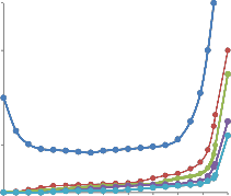
2
the 2-Hop Relay Algorithm is able to support all input rates within the network capacity with finite average delay. However, its delay performance is not necessarily the best. For
example, when the input rate is small (say λ = 0.1 acket /
ot), the average delay is more than 100 slots. Note that the 2-
Hop Relay Algorithm makes scheduling decisions purely based
on the current user locations and restricts all packets to at most
2 hops. It does not attempt to optimize the delay in the network. The delay performance may be improved using alternative scheduling strategies that do not restrict packets to at most 2 hops. For example, backlog aware scheduling and routing (e.g., [7]) or schemes that exploit the mobility pattern of the users (e.g., [15]) may offer better delay performance.
We now investigate the minimum energy function of the cell- partitioned network under consideration. Recall that in our network model, each user either uses zero power or full power. Further, R1 (R2) packets can be transmitted from the sender to the receiver in the same (adjacent) cell if the sender uses full power.
The minimum energy function Φ(λ) is defined as the
minimum time average energy required to stabilize an input
rate λ per user, considering all possible scheduling and routing
1.5
1
0.5
![]()
Analytical
bound for i.i.d. mobility
![]()
x = 0.05
![]() x = 0.1
x = 0.1
![]()
x = 0.25
algorithms that conform to the given network structure. We
exactly compute this function for our network model. Specifically, we assume that all users receive packets at the
same rate (i. e. , λ = λ or a i). Also, we consider the case when
R ≥ 2R (Φ(λ)) for the case when R < 2R has a different
expression, but the proof is similar).
Theorem 3. The minimum energy function 𝛷( ) per user for the
cell-partitioned network as described in Sec. II with ≥ 2 is a
piecewise linear curve given by the following:
0
0.05 0.1 0.15 0.2 0.25 0.3 0.35 0.4 0.45 0.5
Input rate Lambda (Packets/Slot)
![]()
![]()
x = 0.5 i
2 2
Fig. 2. Average packet delay under the 2-Hop Relay Algorithm in a network of 16 cells with 20 nodes for different mixing times of the mobility process.
![]()
Φ( ) =
![]()
![]()
![]()
( 2 ) i
![]()
![]()
1 ( )
( 2 ) i
2 ( ) 2
We next simulate the 2-Hop Relay Algorithm on this network. New packets arrive at each source node according to independent Bernoulli processes, so that a single packet arrives
i.i.d. with probability λ every slot. In Fig. 2, we plot the average
where
![]()
![]()
![]()
{ ( 2 ) i
( )
packet delay vs. λ for different values of x. We also plot the
analytical bound (8) of Theorem 2 for the i.i.d. mobility case (for
which d = 0). It can be seen that the average delay goes to
infinity as λ is pushed closer to the capacity μ = 0.4 acket /
ot (shown by the vertical line in Fig. 2). While the network
capacity is the same for all values of x (since x does not affect
the steady state location distribution), the average delay
increases as x becomes smaller. This is because a smaller x implies a larger value for the parameter d leading to larger delay as suggested by the delay bound (8) in Theorem 2. Thus,![]()
![]()
![]()
0 < , < ,
![]()
![]()
( ) ( )
< and
![]()
( )
<
Thus, the network can stably support users simultaneously
communicating at any rate λ < μ with an energy cost that can be pushed arbitrarily close to Φ(λ) (at the cost of increased
IJSER © 2012 http://www.ijser.org
International Journal of Scientific & Engineering Research, Volume 3, Issue 10, October-2012 9
ISSN 2229-5518
delay). We prove the theorem in 2 parts. First, we establish the necessary condition by deriving a lower bound on the energy cost of any stabilizing algorithm. Then, we establish sufficiency by presenting a specific scheduling policy and showing that the
average delay is bounded under that policy.
opportunities can used is a given cell in a timeslot, the maximum total sum is fixed and hence
= ( ).
![]()
![]()
![]()
Let (x) ∑ , ( )
in (18). Because e̅ ≥ (x), and
Consider any scheduling strategy that stabilizes the system.
Let X (T) denote the number of packets delivered by the
strategy from sources to destinations in time interval (0, T) that
involves exactly ‘a’ same cell and ‘b’ adjacent cell transmissions. For simplicity, assume that the strategy is ergodic and yields
well defined time average energy expenditure per user e̅ and
well defined time average values for x where:
because x ∈ Ω ∩ Ω ∩ Ω ∩ Ω , we have:
� ≥ in �( ) (1 )
∈ ∩ ∩ ∩
Furthermore, for any function g(x) such that g(x) (x) for all
‘x’ and for any set Ω̃ that contains the set Ω ∩ Ω ∩ Ω ∩ Ω , we
have:
( )
![]()
im (1 )
� ≥ in
∈ ̃
( ) (20)
→
The average energy cost per user e̅ of this policy satisfies:
This follows because the function to be minimized is smaller,
and the INFIMUM is taken over a less restrictive set. We now
define four new constraint sets Ω̃ , Ω̃ , Ω̃ , Ω̃ as follows:![]()
![]()
![]()
� ≥ ∑ ( )
,
(1 )
Ω̃ Ω ; Ω̃ Ω ;
This follows by noting that enough packets may not be available during a transmission.
Note that x = 0, and so the only possible non-zero x
variables are for (a, b) pairs that are integers, non-negative, and
such that (a, b) ≠ (0, 0). Let x = (x ) represent the collection of x variables, and note that these variables must satisfy the constraint x ∈ Ω ∩ Ω ∩ Ω ∩ Ω , where the four constraint sets
are defined below:![]()
![]()
Ω̃ { | 2 ∑ } ;
![]()
![]()
![]()
Ω̃ { | 2 ∑ } ;
It can be seen that each of Ω , Ω , Ω , Ω is a subset
of Ω̃ , Ω̃ , Ω̃ , Ω̃ . Therefore, Ω ∩ Ω ∩ Ω ∩ Ω it is a subset![]()
![]()
of Ω̃ ∩ Ω̃ ∩ Ω̃ ∩ Ω̃ . Note that since , we have the
Ω { | ∑ =
( , ) ( , )
1
![]()
} ; Ω { | } ;
following:![]()
![]()
![]()
![]()
1 2 1 2
< <
(21)
![]()
Ω { | ∑ }
![]()
![]()
1
Ω { | ∑ }
where c1 is the maximum rate of source-destination
transmission opportunities in the same cell, c1 + c2 is the
maximum rate of all possible same cell transmission
opportunities and c1 + c2 + c3 is the maximum rate of all same
We now compute four different bounds for e̅, each having the form e̅ ≥ αλ β. These bounds define the four piecewise linear regions of Φ(λ).![]()
![]()
![]()
![]()
1). First note that (x) ≥ ∑ , . This follows from the definition of f(x). Therefore taking g(x) ≥ ∑ , , we
have:![]()
![]()
1
� ≥ in ∑
∈ ̃ ,
cell or source-destination adjacent cell transmission
Because Ω̃ is given by ∑ ,
x = Nλ, the above infimum
opportunities. Here, these quantities are summed over all cells.
Using the definitions of p, q and q from the statement of
Theorem 1, we know that c = C , c c = C ; c c![]()
c = C( q ). For example, (c c c ) can be written as
∑ (X (t) X (t) X (t)) where X (t) is the maximum
number of direct same cell opportunities, X (t) is the maximum
is equal to λ/R . Thus, we have our first linear
constraint for any algorithm that yields a time average
energy of e̅:![]()
� ≥ (22)
number of indirect same cell opportunities given all direct![]()
![]()
2). Next note that (x) ≥ ∑ ,![]()
. This is
opportunities are used and X (t) is the maximum number of
direct adjacent cell opportunities given all same cell
opportunities are used. Since only one of these three![]()
![]()
![]()
because ≥ for any non-n( e, g) a(tiv, )e integer pair
(a, b) such that (a, b) ≠ {(0,0), (1,0)} (using (21)).
Therefore, taking this lower bound of ‘f(x)’ and ‘g(x)’,
IJSER © 2012 http://www.ijser.org
International Journal of Scientific & Engineering Research, Volume 3, Issue 10, October-2012 10
ISSN 2229-5518
we have:![]()
![]()
![]()
2
� ≥ in [ ∑ ]
∈ ̃ ∩ ̃ ,
![]()
![]()
![]()
1 ( )
![]()
![]()
![]()
![]()
= ( 2 ) (24)
4). Finally note that (x) ≥ ∑
( , ) ( , )
The right hand side is equal to the solution of the
following:![]()
![]()
![]()
2
inimi e: ∑ ,
![]()
![]()
![]()
![]()
∑ which follows from the definition of (x) as well as because for all b ≥ 2. Taking this lower bound of (x) as g(x), we have:![]()
![]()
![]()
![]()
![]()
![]()
2 2
� ≥ in [ ∑ ∑ ]
∈ ̃
( , ) ( , )
where Ω̃ = Ω̃ ∩ Ω̃ ∩ Ω̃ ∩ Ω̃ , this is equivalent to the
ubject to: ∑ =
,
following minimization (Using ∑ ,![]()
inimize:
x = Nλ ):![]()
The above optimization is equivalent to minimizing![]()
![]()
![]()
(Nλ x ) subject to c .
The solution is clearly to choose x = R c , and hence
we have:
ubject to:
![]()
![]()
2
∑
![]()
2
( ∑ )
![]()
2
![]()
![]()
![]()
![]()
2 2
� ≥ = (
![]()
![]()
![]()
2 ∑
2 ) (23)
![]()
![]()
![]()
2
∑
![]()
![]()
![]()
![]()
![]()
3). Next we have (x) ≥ ∑ ∑ ,![]()
![]()
which follows from the definition of (x) and because
for all positive b ≥ 1. Thus, taking this lower
bound of (x) as g(x), we have:![]()
![]()
![]()
![]()
![]()
2 1
� ≥ in [ ∑ ∑ ]
∈ ̃ ∩ ̃ ∩ ̃ ,
Letting = ∑ x and simplifying the optimization metric, the above optimization is equivalent to
following:![]()
![]()
![]()
![]()
![]()
![]()
![]()
![]()
1 2 2 2 2 inimize: ( ) ( )
This is equivalent to the following minimization:![]()
inimize:
![]()
2
∑
![]()
1
( ∑ )
![]()
ubject to:
![]()
![]()
2
∑
![]()
ubject to:
![]()
![]()
2
![]()
![]()
![]()
2
The above optimization is solved when x = R c ,
x 2 = R (c c ) and x = R c . Thus have:
2 ( )
![]()
![]()
![]()
� ≥ (2 )
where, we have aggregated the constraint ∑ ,
x = Nλ
2 ( ) 2
into the objective. The coefficients multiplying x10 and
∑ x are both negative, so that the above![]()
![]()
![]()
= ( 2
) (2 )
optimization is solved when x 2 ∑ x =
R (c c ). Similarly, it can be shown that above
optimization is solved when x = R c .These yields:![]()
![]()
![]()
![]()
( )
� ≥ ( 2 )
The necessary sets of conditions for the function Φ(λ)
are obtained by combining these four bounds.
Now we present an algorithm that makes stationary, randomized scheduling decisions independent of the actual
IJSER © 2012 http://www.ijser.org
International Journal of Scientific & Engineering Research, Volume 3, Issue 10, October-2012 11
ISSN 2229-5518
queue backlog values and show that for any feasible input rate
λ < μ, its average energy cost can be pushed arbitrarily close to the minimum value Φ(λ) with bounded delay. However, the
delay bound grows asymptotically as the average energy is
pushed closer to the minimum value. Similar to the capacity achieving 2-Hop Relay Algorithm, this algorithm also restricts packets to at most 2 hops. However, the difference lies in that it greedily chooses transmission opportunities involving smaller energy cost over other higher cost opportunities. An opportunity with higher cost is used only when the given input rate cannot be supported using all of the low cost opportunities.
Thus, depending on the input rate λ, the algorithm uses only a
subset of the transmission opportunities as follows.![]()
1) If 0 λ < , all packets are sent using only
sourcedestination transmission opportunities in the
same cell.
( )
a) Send new Relay packets in same cell: If the transmitter has new packets for its destination, transmit at rate R1. Else remain idle.
b) Send Relay packets to their Destination in same
Note that the above algorithm does not use any adjacent cell transmission opportunities. All packets are sent over at most 2 hops using only same cell transmissions. We now analyze the performance of this algorithm.
cells) as described in Section of “Network model”, with minimum
energy function 𝛷( ) as described above, and user mobility model
as described in Section of “Network model”, the average energy
cost e of the Minimum Energy Algorithm with input rates for
( )
![]()
![]()
2) If λ <
, all packets are sent either using![]()
![]()
each user such that = 𝜌
(where 0 < 𝜌 < 1) and
source-destination transmission opportunities in the same cell or source-relay and relay-destination transmission opportunities in the same cell.
a control parameter 𝛽 (where 1 < 𝛽 < 1 ∕ 𝜌) satisfies:
![]()
� = 𝛷( ) (𝛽 1)𝜌 ( ) (2 )
![]()
![]()
( ) ( )
3) If λ <
, all packets are sent using
same cell transmissions (in either direct transmission or relay modes), or adjacent cell source-destination transmission opportunities.
And the average packet delay 𝐷̅ satisfies:
![]()
( )
![]()
( ) 𝐷̅ 4 2 1
(2 )
4) And finally, when
λ < μ, all transmission
( )𝜌(𝛽 1)
opportunities that restrict packets to at most 2 hops are
used.
To make the presentation simpler, in the following, we only
( )
where B is a constant given by (11) and d is a finite integer that is
related to the mixing time of the joint user mobility process is
given by
![]()
discuss the case where λ <![]()
. The basic idea and![]()
4 ( ) 𝛽
![]()
( )
performance analysis for the other cases are similar.
( )
( )𝜌(𝛽 1)
= [ ]
![]()
![]()
Let λ = ρ
where, 0 < ρ < 1 this is a given
(1 ∕ )
constant. Also define a control parameter β (where 1 < β <
1 ∕ ρ) that is input to the algorithm. This parameter affects an
energy-delay tradeoff as shown in Theorem 4.
1) If there exists, a source-destination pair in the cell, randomly choose such a pair (uniformly over all such pairs in the cell). If the source has new packets for the destination, transmit at rate R1. Else remain idle.
2) If there is no source-destination pair in the cell but there
are at least 2 users in the cell, then with probability βρ,
decide to use the same cell relay transmission
opportunity as described in the next step. Else remain
idle.
3) If decide to use the same cell relay transmission
opportunity in step (2), randomly designate one user
as the sender and another as the receiver. Then with![]()
probability (where 0 < δ < 1 and δ = δ(β) to be
determined later) perform the first action below. Else,
perform the second.
From the above, it can be seen that the control parameter β
allows a (O(β 1), O(1 ∕ (β 1))) tradeoff between the
average energy cost and the average delay bound. Specifically,
the average energy cost e̅ can be pushed arbitrarily close to Φ(λ) by pushing β closer to 1. However, this increases the bound on D̅ as 1⁄(β 1).
Here, we show an example where the network capacity can be strictly improved by making use of network coding in conjunction with the wireless broadcast advantage. Specifically, consider a network with 6 nodes and 4 cells. Suppose the steady state location distribution for all nodes is uniform over
all cells. Thus, π = 1/4 for all c. The one-to-one traffic pairing is given by 1 ↔ 2; 3 ↔ 4; ↔ . Let R1 = 1 and R2 = 0. Thus,
this example only allows same cell transmissions. We further
assume that when a node in a cell transmits, all other nodes in that cell receive that packet. Note that the 2-Hop Relay Algorithm presented in section of “Network capacity” does not make use of this feature.
Using Theorem 1, the network capacity under the model
presented in section of “Network model” can be computed.
IJSER © 2012 http://www.ijser.org
International Journal of Scientific & Engineering Research, Volume 3, Issue 10, October-2012 12
ISSN 2229-5518
![]()
![]()
Specifically, the network capacity is given by μ =![]()
![]()
![]()
![]()
packets/slot per node where θ = and using (2), we have
q = 1 (1 ) and = 1 (1 ) (1 ) .
We now show how network coding can be used to achieve a
throughput that is strictly higher than μ. First we define 4
distinct configurations of the nodes. In configuration I, nodes 1,
4 and 5 are in the same cell and the other nodes can be in any of the remaining cells (but not in the same cell as nodes 1, 4 and 5). Note that this cell can be any one of the 4 cells. From the assumption about the node mobility process, the steady state![]()
![]()
probability of configuration-I is given by υ 4 ( ) ( ) .
In configuration-II, nodes 2, 3 and 5 are in the same cell and the
other nodes can be in any of the remaining cells (but not in the
same cell as nodes 2, 3 and 5). In configuration-III, nodes 2, 4 and 5 are in the same cell and the other nodes can be in any of the remaining cells (but not in the same cell as nodes 2, 4 and 5). Finally, in configuration-IV, nodes 1, 3 and 5 are in the same cell and the other nodes could be in any of the remaining cells (but not in the same cell as nodes 1, 3 and 5). Note that these configurations cannot occur simultaneously as each consists of node 5. Further, the steady state probability of each
configuration is given by υ.
In the following, we will modify the 2-Hop Relay Algorithm
of Sec. III-B when one of these configurations occur in any cell
and demonstrate an improvement in the throughput of nodes 1,
2, 3 and 4 over μ. For each configuration, we will only focus on
the transmissions in the cell with the three nodes that define
that configuration. The 2-Hop Relay Algorithm for the other
cells remains the same.
Note that under each configuration, there are no source- destination pairs in the cell of interest. Thus, under the 2-Hop Relay Algorithm, a node is selected as the transmitter with probability 1/3 while the remaining two nodes are equally likely to be selected as the receiver. Further, the transmitter is scheduled to transmit a new packet to the receiver with![]()
![]()
probability and is scheduled to transmit a relay packet to the receiver with probability . Then, in each configuration,
the two nodes other than node 5 are scheduled to transmit a![]()
![]()
![]()
![]()
new packet to node 5 with probability = . Also,
in each configuration, node 5 is scheduled to transmit a relay
packet to each of the other two nodes in the cell with![]()
![]()
![]()
![]()
probability = .
We now modify the 2-Hop Relay Algorithm to take
advantage of network coding. For all configurations other than
the four as defined above, the algorithm remains the same. However, in each of the configurations-I, II, III and IV, we change the probability of scheduling a node to transmit a new![]()
![]()
![]()
![]()
packet (for relaying) to node 5 from to = where 0![]()
![]()
![]()
< ϵ < 1. Also, node 5 is scheduled to transmit a relay packet to
the other two nodes in the cell with probability = .
However, whenever node 5 has at least one packet for each of
the two other nodes, it broadcasts a XOR of two packets
destined for these nodes in a single transmission. If node 5 does not have at least one packet for each of the two other nodes, it would simply transmit a regular packet (if available). The probabilities associated with the other scheduling decisions under this modified algorithm remain the same as the original
2-Hop Relay Algorithm. It can be seen that the probabilities
under the modified algorithm add to 1.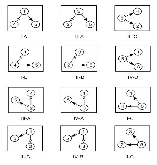
Fig. 3. An example showing capacity gains possible by using network coding in conjunction with the wireless broadcast advantage.
To see how the nodes can recover the original packets from the XOR packet, we further classify each configuration into type A, B and C depending on the scheduling decision as shown in Fig. 3. The configurations of type A and B correspond to the scheduling decisions in which a node is scheduled to transmit a new packet (for relaying) to node 5. The configurations of type C correspond to the scheduling decisions in which node 5 is scheduled to transmit relay packets to the other two nodes (either as a network coded XOR packet whenever possible or a regular packet). In each configuration of type A or B, whenever a new packet is transmitted by a node to node 5 for relaying, the other node overhears the packet and stores a copy. Figure I- A shows, when node 1 transmits a new packet (destined for node 2) to node 5, node 4 overhears this transmission and stores a copy of this packet. Similarly, in II-A, when node 3 transmits a new packet (destined for node 4) to node 5, node 2 overhears this transmission and stores a copy of this packet. In each configuration of type C, whenever node 5 has at least one packet for each of the two other nodes, note that each of these two nodes already has a copy of the packet destined for the other node (that it obtained by overhearing earlier in a type A or B configuration). Therefore, when node 5 transmits a XOR packet, both of these nodes can recover the original packets destined for them by using the side information already available to them in the form of previously overheard and
IJSER © 2012 http://www.ijser.org
International Journal of Scientific & Engineering Research, Volume 3, Issue 10, October-2012 13
ISSN 2229-5518
stored packets. Figure III-C shows, node 5 is in the same cell as nodes 2 and 4 and suppose it has a packet for each of them. Then, node 2 must have the packet that is destined for node 4 that it overheard in II-A. Similarly, node 4 must have the packet that is destined for node 2 that it overheard in I-A. Thus, when node 5 broadcasts a XOR packet in a single transmission, both nodes 2 and 4 can retrieve their desired packets. Thus, this single transmission effectively delivers two packets. Note that under a scheme that does not allow mixing of packets, at most one packet can be transmitted per transmission.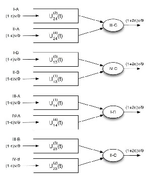
Fig. 4. Additional relay queues at node 5 under the network coding enhanced 2-Hop Relay Algorithm that is used in configurations -I, II, III and IV.
To demonstrate gains in throughput under this “network coding enhanced” 2-Hop Relay Algorithm, we define the following additional relay queues at node 5 as shown in Figure.
4. Arrivals to and departures from these queues happen only when scheduling decisions corresponding to the 12 configurations in Fig. 3 are made according to the enhanced 2-
Hop Relay Algorithm. U ( )(t) & U ( )(t) refer to the queue of
packets destined for nodes i and j respectively that will be
network coded whenever possible. Fig. 4 shows the arrival rates
and the corresponding configurations (when arrivals happen to these queues) as well as the service rates and corresponding configurations (when packets are served from these queues).
( )
capacity can be strictly increased over a scheme that is restricted to pure routing.
In this work, we investigated two quantities of fundamental interest in a delay-tolerant mobile ad hoc network: the network capacity and the minimum energy function. Using a cell- partitioned model of the network, we obtained exact expressions for both these quantities in terms of the network parameters (number of nodes N and number of cells C) and the steady state location distribution of the mobility process. Our results hold for general mobility processes (possibly non- uniform and non-i.i.d.) and our analytical technique can be extended to other models with additional scheduling constraints.
We also proposed two simple scheduling strategies that can
achieve these bounds arbitrarily closely at the cost of an
increased delay. Both these schemes restrict packets to at most 2 hops and make scheduling decisions purely based on the
current user locations and independent of the actual queue backlogs. For both schemes, we computed bounds on the average packet delay using a Lyapunov drift technique.
In this paper, we have focused on network control algorithms that operate according to the network structure as presented in section of “Network model”. We assumed that the packets themselves are kept intact and are not combined or network coded. As shown in the example in section of “Capacity gain by network coding”, it is possible to increase the network capacity by making use of network coding and the wireless broadcast feature. An interesting future direction of this research is to determine the exact capacity region with such enhanced control options.
We are thankful to KamalKiran Tata, Assistant Professor in Department of Electrical and Electronics Engineering of Rise Prakasam Group of institutions, Ongole, AP, India with whom we had useful discussions regarding difficulty in mathematical equations and theorems. Any suggestions for futher improvement of this topic are most welcome.
[1] R. Urgaonkar and M. J. Neely. Capacity region, minimum energy, and delay for a mobile ad-hoc network. Proc. WiOpt, April 2006.
[2] P. Gupta and P. R. Kumar. The capacity of wireless networks. IEEE Trans.
Inform. Theory, vol. 46, no. 2, pp. 388-404, March 2000.
[3] M. Grossglauser and D. Tse. Mobility increases the capacity of ad hoc wireless networks. IEEE Transactions on Networking, vol. 10, no. 4, pp. 477-
486, April 2001.
Note that each queue has an arrival rate of
( )
![]()
and sees a
[4] M. Garetto, P. Giaccone, and E. Leonardi. Capacity scaling in ad hoc
![]()
service rate of
. Since (1 2ϵ) > (1 ϵ), all these queues
networks with heterogeneous mobile nodes: The super-critical regime. IEEE
are stable. The additional throughput for nodes 1, 2, 3 and 4
over the 2-Hop Relay Algorithm without network coding is
( ) ( )
Transactions on Networking, vol. 17, no. 5, pp. 1522-1535, Oct. 2009.
[5] G. Mergen and L. Tong. Stability and capacity of regular wireless networks.
![]()
given by [![]()
] υ packets/slot. This is strictly positive
IEEE Transactions on Information Theory, vol. 51, no. 6, pp. 1938-1953, June
![]()
for any 0 < ϵ < 1/ 4. For example, by choosing ϵ = 1/8, a
throughput gain of packets/slot is achievable. Thus, the
2005.
[6] A. F. Dana, R. Gowaikar, R. Palanki, B. Hassibi, and M. Effros. Capacity of
IJSER © 2012 http://www.ijser.org
International Journal of Scientific & Engineering Research, Volume 3, Issue 10, October-2012 14
ISSN 2229-5518
wireless erasure networks. IEEE Transactions on Information Theory, vol. 52, no. 3, pp. 789-804, March 2006.
[7] M. J. Neely. Dynamic Power Allocation and Routing for Satellite and
Wireless Networks with Time Varying Channels. PhD Thesis, MIT, LIDS,
2003.
[8] M. J. Neely and E. Modiano. Capacity and delay tradeoffs for ad-hoc mobile networks. IEEE Transactions on Information Theory, vol. 51, no. 6, pp. 1917-
1937, June 2005.
[9] S. Toumpis and A. J. Goldsmith. Large wireless networks under fading, mobility, and delay constraints. Proceedings of IEEE INFOCOM, March 2004.
[10] A. El Gammal, J. Mammen, B. Prabhakar, and D. Shah. Throughput delay
trade-off in wireless networks. Proceedings of IEEE INFOCOM, March 2004.
[11] G. Sharma, R. R. Mazumdar and N. B. Shroff. Delay and capacity tradeoffs in mobile ad-hoc networks: A global perspective. Proceedings of IEEE INFOCOM, April 2006.
[12] X. Lin, G. Sharma, R. R. Mazumdar and N. B. Shroff. Degenerate
delaycapacity trade-offs in ad-hoc networks with brownian mobility. Joint Special Issue of IEEE Transactions on Information Theory and IEEE Transactions on Networking, vol. 52, no. 6, pp. 2777-2784, June 2006.
[13] K. Jain, J. Padhye, V. Padmanabhan and L. Qiu. Impact of interference on
multi-hop wireless network performance. Proceedings of ACM MOBICOM, Sept. 2003.
[14] M. Kodialam and T. Nandagopal. Characterizing achievable rates in multi-
hop wireless mesh networks with orthogonal channels. IEEE Transactions on
Networking, vol. 13, no. 4, pp. 868-880, Aug. 2005.
[15] M. Grossglauser and M. Vetterli. Locating nodes with EASE. Proceedings of
IEEE INFOCOM, April 2003.
[16] C. Fragouli and E. Soljanin. Network coding applications. Foundations and
Trends in Networking, NOW Publishers, vol. 2, no. 2, pp. 135-269, 2007.
[17] E. Seneta. Non-negative Matrices and Markov Chains. Springer-Verlag, 1981.
[18] S. Ross. Stochastic Processes. John Wiley & Sons, Inc., New York, 1996.
IJSER © 2012 http://www.ijser.org