
International Journal of Scientific & Engineering Research, Volume 5, Issue 4, April-2014 1574
ISSN 2229-5518
Methods to find improvements in Weather forecast in India (specific to Ahmedabad region)
Rakesh Shah, H M Patel, Avinash Shah, Gaurangi Prajapati , Sanchita Mitra and Anil Kadia
Abstract— This thesis is a contribution to the subjects of midlatitude atmospheric dynamics and targeting observations for the improvement of weather forecasts. For the first time the fullspectrum ofsingular vectors of the Eady model are considered. The importance and implications of the un-shielding and modal unmasking mechanisms to the computed singular vectors are discussed. The computed singular vectors are used to analyse the ver- tical structure of the singular vector targeting function commonly used in observation tar- geting, in a vertical cross-section. Through comparison of this vertical cross-section to the dynamics of singular vectors, inferences about the scale and qualitative behaviour of the perturbations to which particular regions are ’sensitive’ are made. In the final section of the thesis, a new targeting method is introduced. This new targeting method utilises a set of evolved singular vectors to approximate the background errors within the region identi- fied by a set of targeted singular vectors as dynamically connected to the verification re- gion. The two sets of singular vectors can then be used as a computationally inexpensive means of predicting the reduction of forecast error variance that will be obtained from a given deployment of observations. This method differs from previous targeting methods as it makes no use of stationary norms or Kalman filter theory. It allows for both a dy- namically determined estimate of the initial condition errors and allows for the operation- al data assimilation to be taken into account. Another major difference between the new targeting method and existing methods, is that it explicitly predicts the reduction in fore- cast error variance as the difference between the forecast error variance with and without the targeted observations. This additional feature introduces the potential for the predic- tion of instances where adding observations is likely to lead to an increase in t h e fo recas t
er ro r var ia nce in t he ve r ific at io n re gio n.
IJSER © 2014 http://www.ijser.org
International Journal of Scientific & Engineering Research, Volume 5, Issue 4, April-2014
ISSN 2229-5518
1575
Index Terms-Inter anuual Variability,Sea Surfuce Temperature, Rapid Warming,Gulf of Kutch, Gulf ofKhambhat.


•
1-BER IS) 2014
International Journal of Scientific & Engineering Research, Volume 5, Issue 4, April-2014 1576
ISSN 2229-5518
Meteorology is the study of atmospheric phenomena, particularly as a means of forecasting future weather events. Weather forecasts are produced by evolving the estimated current atmospheric state forward in time using large non-linear numerical models of the physical and dy- namical processes in the atmosphere. The ability to create accurate numerical forecasts is reliant on both the accuracy of these models and the accuracy of the initial conditions. The initial conditions used in weather forecasting are statistically based ’compromises’ between observation- al data and a previous forecast, which are generated by a process known as data assimilation. Since Lorenz (1963) brought chaos theory to the attention of meteorologists, it has been understood that the non-linear nature of evolu- tionary process in the atmosphere causes errors (no matter how small) in initial conditions supplied to the forecast models to eventually grow into large errors in the forecast. This chaotic behaviour is referred to as sensitivity to initial conditions and is often summed up with the flippancy “if a butterfly flaps its wings in Brazil a tornado is set off in Texas”. As a direct result of the work of Lorenz (1963), meteorologists began to speculate about the existence of a theoretical upper limits to the times-scales over which an accurate forecast can be made. Since the publication of Lo- renz (1963), improvements in numerical models and obser- vation density have lead to large improvements in forecast accuracy. With the continued development of numerical forecasting methods and new observation platforms, it is hoped that there is still room for improvement before any theoretical limit of predictability is reached.
Since the mid 1990s, there has been a move to make forecast generation methods more specific to the atmospheric flow on a particular day and the requirements of the end user. One part of this move has been the development of methods by which the observa- tion distribution resulting in the most accurate forecast may be objectively determined. With the development of new ’movable’ observation platforms, the possibility of day to day variations in the observation network based on the specific requirements of the forecast may present itself; Emanuel et al. (1995). Observa- tions obtained in this manner have come to be known as ’tar- geted’ or ’adaptive’ observations; Lorenz nd Emanuel (1998). Several questions surround the use of an adaptive observation strategy. Most of these questions are summed up in the words of Thompson (1957):
“What return in increased predictability can be expected from increas- ing the overall density of reporting stations, and how does this com- pare with the corresponding outlay offunds? Where is the point of rap- idly diminishing return per outlay? How should the new stations be located in efecting the increase of overall station density?”
Thompson (1957), however, was writing about the develop- ment of a larger network of fixed ob-servations, and so for ’target- ed’ observations a further question exists: What methods can be used
to identify the best observation locations on a day to day ba- sis? Attempting to answer these questions several targeting methods have already been proposed and tested ’in the field’.
This thesis is a further contribution to the answers to two of these questions, namely,
1. Where should the additional observations be located?
We shall give a more detailed explanation of the subject of adaptive observations. To put the subject of adaptive observa- tions in context, the following section discusses the properties of a ’generic’ weather forecasting system.
2. What method should be applied to identifying these locations?
The production of accurate weather forecasts requires the abil- ity to perform two tasks: Firstly to propagate an estimate of the current atmospheric state forward in time; Secondly to make accurate estimates of the current atmospheric state. The first of these tasks is performed using large numerical weather predic- tion (NWP) models. The second is performed by combining observations of the current state of the atmosphere with an estimate of the atmospheric state from a previous forecast. Hence the additional feature introduces the potential for prediction of instances where adding observations is likely to lead to an increase in the forecast error variation in the verification region.
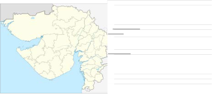
2.1 Area of Study
In and around Ah- medabad, located in the western zone of India , Gujarat.
Ahmedabad is the largest city and former capital of the Indian state of Gujarat.
The city is the administrative headquarters of Ahmedabad district and is the judicial capital of Gujarat as the Gujarat High Court is located here. With a population of more than 5.8 million and an ex- tended population of 6.3 million, it is the fifth largest city and seventh largest metropolitan area of India. It is also ranked third in Forbes' list of fastest growing cities of the decade. Ahmedabad is located on the banks of the River Sabarmati, 32 km (20 mi) from the state capital Gandhinagar.
Though incorporated into the Bombay Presidency during British rule, Ahmedabad remained one of the most important cities in the Gujarat region. The city established itself as the home of a develop- ing textile industry, which earned it the nickname "Manchester of the East". The city was at the forefront of the Indian independence movement in the first half of the 20th century and the centre of many campaigns of civil disobedience to promote farmers' and workers' rights, and civil rights apart from political independence.
IJSER © 2014 http://www.ijser.org
International Journal of Scientific & Engineering Research, Volume 5, Issue 4, April-2014 1577
ISSN 2229-5518
The city has large populations of Hindus, Muslims and Jains, and these cultures are preeminent in the city, with their religious festivals and cuisine dominating the city's culture. Cricket is a popular sport in Ahmedabad, and the Sardar Patel Stadium is situated within the city. In 2012, The Times of India chose Ahmedabad as the best city to live in India.
Map of Gujarat: Coordinates: 23.03°N 72.58°E
ud-din Aybak, in 1451. According to the Bureau of Indian Standards, the town falls under seismic zone-III, in a scale of I to V (in order of increasing vulnerability to earth- quakes) Ahmedabad is divided by the Sabarmati into two physically distinct eastern and western regions. The eastern bank of the river houses the old city, which includes the central town of Bhadra. This part of Ahmedabad is charac- terised by packed bazaars, the pol system of close clustered buildings, and numerous places of worship. It houses the main railway station, the General Post Office, and few buildings of the Muzaffarid and British eras. The colonial period saw the expansion of the city to the western side of Sabarmati, facilitated by the construction of Ellis Bridge in
1875 and later the relatively modern Nehru Bridge. The western part of the city houses educational institutions, modern buildings, residential areas, shopping malls, multi- plexes and new business districts centred around roads such as Ashram Road, C. G. Road & Sarkhej-Gandhinagar Highway.
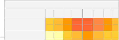
Climate:
![]()
Ahmedabad has a hot semi-arid climate (Köppen climate classification: BSh), with marginally less rain than required for a tropical savanna climate. There are three main sea- sons: summer, monsoon and winter. Aside from the mon- soon season, the climate is extremely dry. The weather is hot through the months of March to June; the average summer maximum is 41 °C (106 °F), and the average min- imum is 27 °C (81 °F). From November to February, the average maximum temperature is 30 °C (86 °F), the aver- age minimum is 15 °C (59 °F), and the climate is extremely dry. Cold northerly winds are responsible for a mild chill in January. The southwest monsoon brings a humid climate from mid-June to mid-September. The average annual rain- fall is about 800 millimetres (31 in), but infrequent heavy torrential rains cause local rivers to flood and it is not un- common for droughts to occur when the monsoon does not extend as far west as usual. The highest temperature rec- orded is 48.5 °C (119.3 °F).
Ahmedabad is located at 23.03°N 72.58°E in western In- dia at an elevation of 53 metres (174 ft) from sea level on the banks of the Sabarmati river, in north-central Gujarat. It covers an area of 464 km2 (179 sq mi).
The Sabarmati frequently dries up in the summer, leaving only a small stream of water, and the city is lo
Climate data for Ahmedabad (1971–
Month Jan Feb Mar Apr May Jun Jul Aug
sandy and dry area. The steady expansion of th
Kutch threatens to increase desertification arou
area and much of the state. Except for the sAverage high °C (°F) 28.3
30.4
35.6
39.8
41.5
38.4
33.4
31.8
of Thaltej-Jodhpur Tekra, the city is almost flat. are within the city's limits—Kankaria Lake and
(82.9) (86.7)
(96.1) (103.6) (106.7) (101.1) (92.1) (89.
Lake. Kankaria lake, in the neighbourhood ofMa Daily mean °C (°F) 20.1 22.2 27.3 31.7 33.9 32.8 29.5 28.2
an artificial lake developed by the Sultan of Delhi, Qutb-
IJSER © 2014 http://www.ijser.org
International Journal of Scientific & Engineering Research, Volume 5, Issue 4, April-2014 1578
ISSN 2229-5518
(68.2) (72) (81.1) (89.1) (93) (91) (85.1)3 (82S.8E)CT(I8O4N.4S) (83.3) (76.5) (70.3) (81.4)
The climate of India resolves into six major climatic sub-
11.8
13.9
18.9
23.7
26.2
27.2
25.6 types; their influences give rise to desert in the west,alpine
age low °C (°F)
(53.2) (57)
(66)
(74.7)
(79.2)
(81)
(78.
tundra and glaciers in the north, humid tropical regions
supporting rain forests in the southwest, and Indian Ocean
all mm (inches)
2 1 0 3
20 103
247
island territories that flank theIndian subcontinent. Regions
(0.08) (0.04)
(0)
(0.12)
(0.79)
(4.06)
(9.7
have starkly different—yet tightly clustered—
microclimates. The nation is largely subject to four sea-
rainy days (≥ 0.1 mm) 0.3 0.3 0.1 0.3 0.9 4.8 13.6 sons: winter (January and February), summer (March to
May), a monsoon (rainy) season (June to September), and a
post-monsoon period (October to December).
monthly sunshi ne hours 288.3 274.4 279 297 328.6 237 130.
e: HKO[33]
Effects of climate change :
Following a heat wave in May 2010, reaching 46.8
°C (116.2 °F), which claimed hundreds of lives, the Ah- medabad Municipal Corporation (AMC) in partnership with an international coalition of health and academic groups and with support from the Climate & Development Knowledge Network, has developed the Ahmedabad Heat Action Plan. Aimed at increasing awareness, sharing in- formation and coordinating responses in order to reduce the health effects of heat on vulnerable populations, the action plan is the first comprehensive plan of its kind in India.
2.4 Copyright Form
An IJSER copyright form must accompany your final submission. You can get a .pdf, .html, or .doc version at http://computer.org/copyright.htm. Authors are responsible for obtain- ing any security clearances.
For any questions about initial or final submission requirements, please contact one of our staff members. Contact information can be found at: http://www.ijser.org.
————————————————
• Rakesh is currently pursuing doctoral degree program in mathematics in
Pacific University, India,.
• H M Patel is currently Head of Department in Mathamatica Department in
Bhavan’ss College, India,
India's geography and geology are climatically pivotal: the Thar Des ert in the northwest and the Himalayas in the north work in tandem to effect a culturallyand economically break-all monsoonal regime. As Earth's highest and most massive mountain range, the Himalayan system bars the influx of frigidkatabatic wind- s from the icy Tibetan Plateau and northerly Central Asia. Most of North India is thus kept warm or is only mildly chilly or cold during winter; the same thermal dam keeps most regions in India hot in summer.
Though the Tropic of Cancer—the boundary between the tropics and subtropics—passes through the middle of India, the bulk of the country can be regarded as climatically trop- ical. As in much of the tropics, monsoonal and other weather patterns in India can be wildly unstable: epochal droughts, floods, cyclones, and other natural disasters are sporadic, but have displaced or ended millions of human lives. There is widespread scientific consensus that South Asia is likely to see such climatic events, along with their aleatory unpredictability, to change in frequency and are likely to increase in severity. Ongoing and future vegetative changes and current sea level rises and the attendant inun- dation of India's low-lying coastal areas are other impacts, current or predicted, that are attributable to global warming.
Tectonic movement by the Indian Plate caused it to pass over a geologic hotspot—the Réunion hotspot—now occu- pied by the volcanic island ofRéu nion. This resulted in a massive flood basalt event that laid down the Deccan Trap- s some 60–68 Ma, at the end of the Cretaceous period. This may have contributed to the global Cretaceous–Paleogene extinction event, which caused India to experience signifi- cantly reduced insolation. Elevated atmospheric levels of sulphur gases formedaer osols such as sulphur diox- ide and sulphuric acid, similar to those found in the atmosphere of Venus; these precipitated as acid rain. Elevated carbon dioxide emissions also contributed to the greenhouse effect, causing warmer weather that lasted
IJSER © 2014 http://www.ijser.org
International Journal of Scientific & Engineering Research, Volume 5, Issue 4, April-2014 1579
ISSN 2229-5518
long after the atmospheric shroud of dust and aerosols had cleared. Further climatic changes 20 million years ago, long after India had crashed into the Laurasian landmass, were severe enough to cause the extinction of many endemic Indian forms. The formation of the Himalayas resulted in blockage of frigid Central Asian air, preventing it from reaching India; this made its climate significantly warmer and more tropical in character than it would otherwise have been.
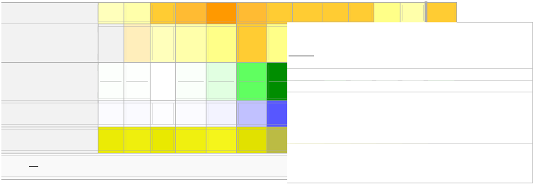
four-season classification scheme used by the IMD;[N
1] year-round averages and totals are also displayed.
The India Meteorological Department (IMD) designat • Badger, J., and B. J. Hoskins, 2001: Simple Initial
four climatological seasons:
• Winter, occurring from December to March. The year's coldest months are December and January•,
when temperatures average around 10–15 °C (50–59 °F) in the
northwest; temperatures rise as one proceeds towards the equator, peaking around 20–25 °C (68–77 °F) in mainland India's southeast.
• Summer or pre-monsoon season, lasting from April to June (April to July in northwestern India). I•n western and southern regions, the hottest month is April; for northern
regions, May is the hottest month. Temperatures average around 32–
40 °C (90–104 °F) in most of the interior.
• Monsoon or rainy season, lasting from July to September. The season is dominated by the humid southwest summer monsoon, which slowly sweeps across the cou
Value Problems and Mechanisms for Baroclinic
Growth. J. Atmos. Sci., 1, 38–49.
Barkmeijer, J., M. Van Gijzen, and F. Bouttier, 1998: Singular vectors and estimates of the analysis-error covariance metric. Quart. J. Roy. Meteor. Soc,
Bergot, T., 2001: Influence of the assimilation scheme on the efficiency of adaptive observations.Quart. J. Roy. Meteor. Soc, 127, 635–660.
try beginning in late May or early June. Monsoon rains begin to r • ^ Meteorology b y Lisa Alter
cede from North India at the beginning of October. South India ty
cally receives more rainfall.
• Post-monsoon or autumn season, lasting from October through November. In northwestern India, O tober and November are usually cloudless. Tamil Nadu receives mo of its annual precipitation in the northeast monsoon season.
The Himalayan states, being more temperate, experience additional season, spring, which coincides with the fir weeks of summer in southern India. Traditionally, India
• Weather: Forecasting from the Beginning
• University of California Museum of Paleontology. Aristotle (384-
322 B.C.E.). Retrieved on 2008-01-12.
• David Pingree. "THE INDIAN AND PSEUDO-INDIAN PASSAG- ES IN GREEK AND LATIN ASTRONOMICAL AND ASTRO- LOGICAL TEXTS". pp. 141–195 [143–4]. Retrieved 2010-03-01
note six seasons or Ritu, each about two months lon • Fahd, Toufic. "Botany and agriculture". p. 842, in Rashed, Roshdi;
These are the spring season (Sanskrit: vasanta), summ (grīṣma), monsoon season (varṣā), autumn (śarada), wint (hemanta), and prevernal season[24](śiśira). These are bas on the astronomical division of the twelve months into s
Morelon, Régis (1996).Encyclopedia of the History of Arabic Scien- ce 3. Routledge. pp. 813–852. ISBN 0-415-12410-7
parts. The ancient Hindu calendar also reflects these se • ^ Kalman, R.E. (1960). "A new approach to linear filtering and
sons in its arrangement of month.

Shown below are temperature and precipitation data for
prediction problems". Journal of Basic Engineering 82 (1): pp. 35–45
• Steffen L. Lauritzen. "Time series analysis in 1880. A discussion of contributions made by T.N. Thiele".International Statistical Re- view 49, 1981, 319–333.
selected Indian cities; these represent the full variety of m • Steffen L. Lauritzen, Thiele: Pioneer in Statistics, Oxford University
jor Indian climate types. Figures have been grouped by th
Press, 2002. ISBN 0-19-850972-3.
IJSER © 2014 http://www.ijser.org
International Journal of Scientific & Engineering Research, Volume 5, Issue 4, April-2014 1580
ISSN 2229-5518
The production of accurate weather forecasts requires the ability to perform two tasks: Firstly to propagate an estimate of the current atmospheric state forward in time; Secondly to make accurate esti- mates of the current atmospheric state. The first of these tasks is per- formed using large numerical weather prediction (NWP) models. The second is performed by combining observations of the current state of the atmosphere with an estimate of the atmospheric state from a previous forecast.
The second task required for the successful production of a forecast needs slightly more explanation. Ideally the model would be initial- ized using a set of homogeneously distributed accurate observations, at least equal in number to the number of variables in the model state vector χ. Unfortunately, due to the high dimension of the model state and the inaccessibility of many required observation locations, the observations are neither large enough in number nor homo-geneous enough in their distribution to specify entirely the model state. In order to solve this problem the observational data are combined with a previous forecast to produce the estimated current atmospheric state, χa, based on the estimated statistics of the error in both the fore- cast and observations. This process is known as data assimilation. The forecast used in the data as-similation process is known as the background. The estimated state obtained through the data assimila- tion process is known as the analysis.
where χ is a vector containing the model state variables (pressure, temperature, velocity at different grid points for example) and M is a non-linear operator con- taining the model equations.
The various data assimilation methods in use in weather forecasting centres derive from the minimisation of the quadratic cost function:
where the vector χ is the control vector1, χb is a vector containing the background, y is a vector containing the observations, H is the forward model (or observation operator) which transforms the model variables to the observed variables R is matrix containing an estimate of the covariance between observational errors, and B is a matrix containing an estimate of the covariance between the errors in the background. From this cost function the analysis χa can be defined as the vector χ for which J(χ) is minimised. In order to formulate the cost function, certain as- sumptions have to be made about the background and observation errors. These assumptions are, that the observation and background errors are statistically inde- pendent, and that individually the assumed error statistics must lead to non- singular covariance matrices. The assumption of non-singular covariance matri- ces essentially implies that all possible states must have a reasonable probability of existing, even if in the current atmospheric flow they are so unlikely that their probability of existing is very close to zero. A useful property of the cost function is that if the approximation to
the background and observation errors is ’good’ and the forward model can be approximated by the linear operator H, the analysis error covariance matrix A is equal to the inverse of the Hessian (second derivative with respect to χ) of the cost function; i.e(1).
A= [δ2J/ δ x2]-1=[B-1 +HT R-1H]-1
Ideally the covariance matrices in the cost function would depend on the time of observation and the observations would be used to correct the model state corre- sponding to the time of observation. To make the background error covariance time specific one could in theory evolve the analysis error covariance matrix. In reality however the dimension of the model state vector is typically greater than
106 so that the background error covariance cannot be stored by current comput-
ers, let alone evolved or explicitly inverted. Due to the limitations in computation- al power and concerns that evolving covariance matrices may become singular, many methods of solving approximate cost functions have been developed.
6.1 Figures and Tables
Because IJSER staff will do the final formatting of your paper, some figures may have to be moved from where they appeared in the orig- inal submission. Figures and tables should be sized as they are to appear in print. Figures or tables not correctly sized will be returned to the author for reformatting.
Detailed information about the creation and submission of images for articles can be found at: http://www.ijser.org. We strongly encour- age authors to carefully review the material posted here to avoid problems with incorrect files or poorly formatted graphics.
Place figure captions below the figures; place table titles above the tables. If your figure has two parts, include the labels “(a)” and “(b)” as part of the artwork. Please verify that the figures and tables you mention in the text actually exist. Figures and tables should be called out in the order they are to appear in the paper. For example, avoid referring to figure “8” in the first paragraph of the article un- less figure 8 will again be referred to after the reference to figure 7. Please do not include figure captions as part of the figure. Do not put captions in “text boxes” linked to the figures. Do not put borders around the outside of your figures. Per IJSER, please use the abbreviation “Fig.” even at the beginning of a sentence. Do not abbreviate “Table.” Tables are numbered numerically.
Figures may only appear in color for certain journals. Please veri- fy with IJSER that the journal you are submitting to does indeed accept color before submitting final materials. Do not use color un- less it is necessary for the proper interpretation of your figures.
Figures (graphs, charts, drawing or tables) should be named fig1.eps, fig2.ps, etc. If your figure has multiple parts, please submit as a single figure. Please do not give them descriptive names. Author photograph files should be named after the author’s LAST name. Please avoid naming files with the author’s first name or an abbreviat- ed version of either name to avoid confusion. If a graphic is to appear in print as black and white, it should be saved and submitted as a black and white file (grayscale or bitmap.) If a graphic is to appear in color, it should be submitted as an RGB color file.
The first of the two targeting methods that were used in the At REC
field experiment is the singular vector method. In simplistic terms the essential components of the singular vector method can be sum-
IJSER © 2014 http://www.ijser.org
International Journal of Scientific & Engineering Research, Volume 5, Issue 4, April-2014 1581
ISSN 2229-5518
marised thus: A small set of perturbations (the singular vectors) that maximise the amplification of small perturbations to the initial con- ditions over the finite forecast integration period are calculated; the observations are then targeted to regions in which this set of pertur- bations weighted by their amplification over the forecast period have large amplitude. The finer details of this method are somewhat more complex than this simplistic explanation so we shall break it down into three sections. Firstly we shall describe the mathematical prop- erties and computation of the singular vectors. Secondly we shall describe the implementation of the targeting method using the singu- lar vectors. Finally we shall identify some assumptions that may be used to link the method to the generic description of ’A-optimal’ targeting methods.
6.3 Footnotes
Number footnotes separately in superscripts (Insert | Footnote)1. Place the actual footnote at the bottom of the column in which it is cited; do not put footnotes in the reference list (endnotes). Use letters for table footnotes (see Table 1). Please do not include footnotes in the abstract and avoid using a footnote in the first column of the article. This will cause it to appear of the affiliation box, making the layout look confus- ing.
6.4 Lists
The IJSER style is to create displayed lists if the number of items in the list is longer than three. For example, within the text lists would appear 1) using a number, 2) followed by a close parenthesis. How- ever, longer lists will be formatted so that:
1. Items will be set outside of the paragraphs.
2. Items will be punctuated as sentences where it is appropriate.
3. Items will be numbered, followed by a period.
300 E to 330 E during 1s t 7t h January 2006. The numbers
in parenthesis compare only those results calculated at locations and days simulated in each case.
7.1 Appendices
Appendixes, if needed, appear before the acknowledgment. In the event multiple appendices are required, they will be labeled “Appendix A,” “Appendix B, “ etc. If an article does not meet submission length re- quirements, authors are strongly encouraged to make their appendices supplemental material.
IJSER Transactions accepts supplemental materials for review with regular paper submissions. These materials may be published on our Digital Library with the electronic version of the paper and are available for free to Digital Library visitors. Please see our guidelines below for file specifications and information. Any submitted materials that do not follow these specifications will not be accepted. All materials must follow US copyright guidelines and may not include material previously copyrighted by another author, organization or company. More information can be found at http://www.ijser.org.
7.2 Acknowledgments
I would like to thank my superiors for assisting me in my studies.I am thankful to Dr H M Patel , Ms Sanchita Mitra for being helpful and kind in giving me assistance.
7.3 References
Table 7.1: Results showing the mean, RMS, and STD of
0 0 1 5 m S E V I R I , i n C , for the area 45 N to 25 N and
1It is recommended that footnotes be avoided (except for the unnumbered footnote with the receipt date on the first page). Instead, try to integrate the footnote information into the text.

manuscript is the order they will appear in the final paper, i.e., refer- ences submitted nonalphabetized will remain that way.
Please note that the references at the end of this document are in the preferred referencing style. Within the text, use “et al.” when referencing a source with more than three authors. In the reference section, give all authors’ names; do not use “et al.” Do not place a space between an authors' initials. Papers that have not been pub- lished should be cited as “unpublished” [4]. Papers that have been submitted or accepted for publication should be cited as “submitted for publication” [5]. Please give affiliations and addresses for per- sonal communications [6].
Capitalize all the words in a paper title. For papers published in transla-
tion journals, please give the English citation first, followed by the original foreign-language citation [7].
7.3 Additional Formatting and Style Resources
Additional information on formatting and style issues can be obtained in the IJSER Style Guide, which is posted online at: http://www.ijser.org/. Click on the appropriate topic under the Special Sections link.
IJSER © 2014 http://www.ijser.org
International Journal of Scientific & Engineering Research, Volume 5, Issue 4, April-2014 1582
ISSN 2229-5518

For the first time the full spectrum of sin
ta" (PDF), Current Science 91(8): 1085–1089, retrieved 1 October
2011
gular vectors of theEady model are consid• BAGLA, P. (2006), "Controversial Rivers Project Aims to Turn India's
Fierce Monsoon into a Friend",Science (August 2006) 313 (5790):
ered. The importance and implications
the unshielding and modal unmaskin
1036–1037, doi:10.1126/science.313.5790.1036,ISSN 0036-
8075, PMID 16931734
mechanisms, to the computed singular vec• BLASCO, F.; BELLAN, M. F.; AIZPURU, M. (1996), "A Vegetation Map
tors are discussed. The computed singula vectors are used to analyse the singula
of Tropical Continental Asia at Scale 1:5 Million", Journal of Vege- tation Science (Journal of Vegetation Science, published October
1996) 7 (5): 623–634, doi:10.2307/3236374, JSTO R 3236374
vector targeting function commonly used i • BURNS, S. J.; FLEITMANN, D.; MATTER, A.; KRAMERS, J.; AL-
observation targeting, in a vertical cross section.
![]()
We wish to thank our departmetnfor allowing us to do this extensi work and finally conclude the thesis, also my family and friends.
• Steffen L. Lauritzen. "Time series analysis in 1880. A discussion of contributions made by T.N. Thiele".International Statistical Re- view 49, 1981, 319–333.
• Steffen L. Lauritzen, Thiele: Pioneer in Statistics, Oxford University
Press, 2002. ISBN 0-19-850972-3.
• Stratonovich, R.L. (1959). Optimum nonlinear systems which bring about a separation of a signal with constant parameters from noise. Radiofizika, 2:6, pp. 892–901.
• ALI, A. (2002), "A Siachen Peace Park: The Solution to a Half- Century of International Conflict?",Mountain Research and Devel- opment (November 2002) 22 (4): 316–319, doi:10.1659/0276-
4741(2002)022[0316:ASPPTS]2.0.CO;2, ISSN 0276-4741
• BADARINATH, K. V. S.; CHAND, T. R. K.; PRASAD, V. K.
(2006), "Agriculture Crop Residue Burning in the Indo-Gangetic
Plains—A Study Using IRS-P6 AWiFS Satellite Da-
SUBBARY, A. A. (2003), "Indian Ocean Climate and an Absolute
Chronology over Dansgaard/Oeschger Events 9 to
13", Science 301 (5638): 635–
638,Bibcode:2003Sci...301.1365B, doi:10.1126/science.1086227, IS SN 0036-8075,PMID 12958357
• C. W. Fairall, E. F. Bradley, J. S. Godfrey, G. A. Wick, J. B. Edson, and G. S. Young. Cool-skin and warm-layer eects on sea sur- face temperature. J. Geophys. Res.,
101:12951308, 1996.
• C. W. Fairall, E. F. Bradley, J. E. Hare, A.
A. Grachev, and J. B. Edson. Bulk parame- terization of air-sea uxes: Updates and ver- ication for the COARE algorithm. J. Cli- mate, 16:571591, 2003.
IJSER © 2014 http://www.ijser.org