International Journal of Scientific & Engineering Research, Volume 5, Issue 12, December-2014 1330

ISSN 2229-5518

Methods for Crime Analysis Using GIS

Shahebaz M. Ansari, Dr. K. V. Kale

Abstract— Geographic Information System (GIS) is a fast growing technology where one can make the use of digital Maps and spatial data for visualizing, analyzing and taking decision based on the analysis. It can also be use for mapping and analyzing the crime and its impact. Mapping of Crime using GIS technology can be effective in Emergency situations. Hotspots of particular crime incident can be identified for finding its intensity and for taking effective decision. Kernel Density Estimation, Getis-Ord Gi*, Moran’s I, IDW and different other methods can be used for finding the Hotspot which are discussed in this paper so that one can select the appropriate methods according to the requirement which can be of crime, forestry, tourist management, emergency crisis, wildlife reserve and many others.

Index Terms— Crime Analysis, Getis-Ord Gi*, GIS, Hot Spot, IDW, KDE, Moran’s I

——————————  ——————————

1 INTRODUCTION

computer framework which is used for capturing, pre- serving, querying, exploring and displaying geospatial data is known as Geographic Information System (GIS).
The Geospatial data also known as geographically referenced data describes both the location and the characteristics of the feature called spatial feature which may consist of roads, land extents, and vegetation on the Earth surface [1] [2] [3]. The thing that differentiates GIS from other information system is its capability of handling and performing operations on Geo- spatial data. The spatial data may be the location while the attribute data is the characteristics possessed by that location [1]. GIS derived as an economical tool for various applications over the past decade. It is applied for emergency movement and transportation management [3] [4]. GIS has come up with information management and mapping, which have its roots in modeling and analysis which facilitates decision making [5].
Crime is any practice performed by an individual or a group of individuals which is unethical, harmful and unsocial to the society. Crime can be the result of illiteracy, poverty, or revenge. Criminal activity from a long time ago is the matter of worry in contemporary society. Many countries in the world are facing intolerable level of crime and delinquency [6]. Crime analysis is the qualitative and quantitative aspect of acquiring the knowledge of crime and law enforcement in- formation posses with social-statistics and spatial circum- stances to understand criminals, reduce public disturbance and prevent crime [2]. It describes the methodological collec- tion, preparation, and understanding and makes publically the information related to criminal activity to support the task of law enforcement [7] [8].
The concept of crime mapping and analysis and Hotspot Detection techniques can also be used for forest fire preven- tion by finding out the place where maximum fire broke and

————————————————

• Shahebaz M. Ansari is currently pursuing Masters Degree program (M.Tech. in Computer Science and Engineering) in Dr. Babasaheb Ambedkar Marathwada University, Aurangabad (MS), India, Mob.-

+919881077786. E-mail: shahebaz.a@gmail.com

• Dr. K. V. Kale is the Professor at Department of Computer Science and IT

in Dr. Babasaheb Ambedkar Marathwada University, Aurangabad (MS), India, PH-(+91240) 240043222. E-mail: kvkale91@gmail.com
can carry out measures to prevent it. Similarly in Vehicle or Auto-theft incidence it can be used to find the area where maximum theft has occurred and also find its pattern to take appropriate action. In Tourist Management area by providing the mostly crowded place and adding temporal phenomenon with it will be helpful for tourist for identifying the area where a particular crime is more so that they can take precautions and opt for different options in new states or country.
GIS provides with a vast variety of solutions for our day to day problems which may range from finding nearest facili- ties, shortest distance to reach the desires facility or place, providing alternate routes in traffic jam, communicating your location in emergency situations and may more. It can be used according to the area of interest and can be framed for ensur- ing the effective and efficient output from it.
Crime analysis helps police agencies to solve the crimes, develop effective strategies and tactics to prevent future crimes. It also helps in finding and apprehending offenders and also prosecuting and convicting them. GIS can improve safety and quality of life, optimize internal operations; priori- tize patrol and investigations. It can be used to detect and solve community problems, allocate resources, plan for future resource needs and enact effective policies [9].

1.2 Hot Spot

The term hot spot has become an integral part of the study called crime analysis and is popular with most of the analyst. A hot spot as the name suggests is a state of indicating some arrangements of clusters in a spatial distribution [8]. The clus- ter of geographical areas consisting of habitually high number of crime events are known as Hotspots [10]. Crime hot spots can be considered to be place of high crime intensity. Getting the knowledge of concentration of crime law enforcement agencies can make timely and effective decisions about ap- pointing police resources. In addition, crime hot spots mapped by GIS can impressively communicate crime patterns and crime prevention policies to decision makers and the public [11].
GIS based hot spot identification in the criminal cases is to

International Journal of Scientific & Engineering Research, Volume 5, Issue 12, December-2014 1331

ISSN 2229-5518

precisely state the characteristics of criminal activity occurred and its distribution over the area. This can be used as a the- matic map for the user [12]. The Hot Spot Analysis tool identi- fies spatial clusters of statistically significant high or low at- tribute values [13]. One has to provide a set of data values, which may be the number of crimes per area, expecting that the data values are randomly spread across the study area, this tool provide clusters of census blocks with crime incidents higher than expected. These clusters so formed are hot spots. The Hot Spot Analysis tool also provides spatial clusters of crime incidents lower than expected. These clusters reproduce crime cold spots and it may also provide facts about policy or environmental circumstances that deter crime [11].

2 LITERATURE REVIEW

The GIS technology as a tool can be effectively used to solve our day-to-day problems and help us to have a compact yet effective solution to our queries. It supports network anal- ysis and planning whether it may be a Road network or a network of Stream. The GIS technology can be used according to the field of interest and the problem domain [4] [5].
The GIS and Remote Sensing can be used for visualizing the data, analyzing the facts, and to take firm decision based on the analysis. This can be used to map the Police stations and to identify the Crime Zone as Hot Spot and to statistically analyze the reported Crime which will help to take effective measures to control the crime [9].
The Hot Spot methods in Crime analysis can be broadly classified as shown in Fig. 2.1 into three categories, namely Spatial Analysis Methods, Interpolation Methods and Map- ping Cluster or Spatial Interpolation Methods [1] [14]. Differ- ent Methods used for Hotspot detection are as follows: [15]
• Spatial Analysis Methods:

o Kernel Density Estimation

• Interpolation Methods:

o Inverse distance weighted (IDW) interpolation

o Kriging

o Spline

o Natural Neighbor

• Mapping Cluster

o Cluster and Outlier Analysis (Anselin Local

Moran's I)

o Hot Spot Analysis (Getis-Ord Gi*)

2.1 Spatial Analysis Method

Spatial Analysis is the process of checking the locations, at- tributes, and connection of features in spatial data among overlay and other analytical techniques; which is used for ac- quiring knowledge that can be used in different aspect. Spatial
analysis creates or extracts different new information from spatial data [15]. Different techniques under this category are Kernel Density Estimation (KDE) [16] [17], Point Density [17], Line Density.

2.2 Interpolation Methods

Interpolation is the process of using points with better- known values to propose values at alternate unknown points. It is often used to foretell unknown values at any geo- graphic point data, which can be used in the field of rainfall, noise levels, chemical concentrations, elevation, or other spa- tially-based phenomena. It is the approximate judgment of surface values at the points which are un-sampled based on the surface values of surrounding points which are known. Interpolation is usually used as a raster operation, but using a TIN (Triangulated Irregular Networks) surface model it can be used as vector operation [15] [18]. There are several well- known interpolation techniques such as Inverse Distance Weighted (IDW), Kriging, Spline, and Natural Neighbor.

2.3 Mapping Cluster

Mapping Cluster also known as Spatial Autocorrelation is an amount of the degree to which a set of spatial features and the data values associated with it. It can be clustered together in Space (positive spatial autocorrelation) or Scatter Widely (negative spatial autocorrelation) [15]. Different methods un- der Mapping Cluster or Spatial Autocorrelation are Anselin Local Moran's I [13] [16] and Getis-Ord Gi* [1].

3 CRIME ANALYSIS METHODS

Different methods for crime analysis and hotspot detection are discussed. Mathematical notations of each technique are also given to provide full understanding of the input, output and working or the functioning of the technique. These methods can be used for analysis and making decisions as per the situa- tion and requirement [1] [13] [14].

3.1 Kernel Density Estimation (KDE)

Density Estimation measures cell densities in a raster by using a sample of known points. There are two variants known as Simple Density and Kernel Density Estimation methods. For Simple Density Estimation method, we have to place a raster on a point distribution, then arrange points that fall within each cell, sum the point values and estimate the cell’s density by dividing the total point value by the cell size [16] [17].

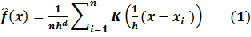
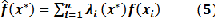
For the purpose of estimation the Kernel Density Estima- tion associates each known point with a Kernel function. This can be expressed as a bivariate probability density function, a kernel function looks like a “bump”, centering at a known point and tapering off to 0 over a defined bandwidth or win- dow area. The kernel function and the bandwidth determine the shape of the bump, which in turn determines the amount of smoothing in estimation [19]. The Kernel Density Estima- tion at point is then the sum of bumps placed at the known
points within the bandwidth:

International Journal of Scientific & Engineering Research, Volume 5, Issue 12, December-2014 1332

ISSN 2229-5518

where is the kernel function, is the bandwidth, is the number of known points within the bandwidth, and is the data dimensionality. For two-dimensional data ( ),

the kernel function is usually given by:
By substituting Eq. 2 for , Eq. 1 can be rewritten as:
where is a constant, and and
are the deviation in x-, y-coordinates between point and
known point that is within the bandwidth. Density values
in the raster are expected values rather than probabilities. Kernel Density Estimation usually produces a smoother sur- face than the simple estimation method does [1] [20] [21] [22]

[23] [24] [25] [26] [27] [28].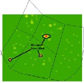
(a) (b)
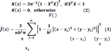
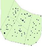
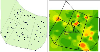
Figure 3.1 Figure (a) shows the Crime Incidents and (b)
shows the KDE opertation on (a)
The Fig. 3.1 (a) shows the crime events in and (b) shows the Hot Spot detected after applying KDE on it. The Hot Spots found are circled in (b) for making it understandable.

3.2 Inverse Distance Weighted (IDW) Interpolation Inverse Distance Weighted (IDW) Interpolation is an exact method that enforces the condition that the estimated value of

a point is influenced more by nearby known points than by
those farther away. The general equation for the IDW method

is:

where is the estimated value at point 0, is the value at known point , is the distance between point and point 0, is the number of known points used in estima-
tion, and is the specified power [1].
The power controls the degree of local influence. A power of 1.0 means a constant rate of change in value between points (linear interpolation). A power of 2.0 or higher suggests that the rate of change in values is higher near a known point
as compared to other points. The degree of local influence also
depends on the number of known points used in estimation. In IDW all the predicated values are within the range of max- imum and minimum values of the known points [1] [7] [22] [29].

(a) (b)
Figure 3.2 (a) shows the Crime Incidents and (b) shows the
IDW opertation on (a)
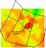
The Fig. 3.2 (a) shows the crime events and (b) shows the Maximum crime area identified by applying IDW operation on it. The circle shows the detected Hot Spot.

3.3 Kriging

Kriging is an advanced Geostatistical procedure that generates an estimated surface from a scattered set of points with - values. Unlike other interpolation methods, Kriging effective- ly involves an interactive investigation of the spatial behavior of the phenomenon represented by the -values before you select the best estimation method for generating the output surface [30].
Kriging assumes that the distance or direction between sample points reflects a spatial correlation which can be used to explain variation in the surface. The Kriging tool fits a mathematical function to a specified number of points, or all points within a specified radius, to determine the output value for each location. Kriging is a multistep process; it includes exploratory statistical analysis of the data, variogram model- ing, creating the surface, and (optionally) exploring a variance surface. Kriging is most appropriate when you know there is a spatially correlated distance or directional bias in the data. It is often used in soil science and geology [31]. Kriging is similar to IDW in that it weights the surrounding measured values to derive a prediction for an unmeasured location. The general formula is given as:

In IDW, the weight, , depends solely on the distance to the prediction location. However, with the Kriging method, the weights are based not only on the distance between the measured points and the prediction location but also on the
overall spatial arrangement of the measured points. To use the spatial arrangement in the weights, the spatial autocorrelation must be quantified. Thus, in ordinary Kriging, the weight , depends on a fitted model to the measured points, the distance

International Journal of Scientific & Engineering Research, Volume 5, Issue 12, December-2014 1333

ISSN 2229-5518

to the prediction location, and the spatial relationships among the measured values around the prediction location [1] [7].
(a) (b)
Figure 3.3 (a) shows the Crime Incidents and (b) shows the
Kriging opertation on (a)
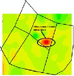
The Fig. 3.3 (a) shows the crime events and (b) shows the Maximum crime area or Hot Spot formed after applying Kriging operation; within the circled area.

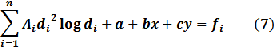
3.4 Thin-Plate Splines

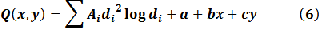
Splines for spatial interpolation are conceptually similar to Splines for line smooting except that in spatial interpolation they apply to surfaces rather than lines. Thin-plate Splines create a surface that passes through the control points and has the least possible change in slope at all points. The
approximation of Thin-plate Splines is of the form:

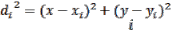
where x and y are the x-coordinate and y-coordinate of the point to be interpolated, and and are the x-, y-coordinates of control point .
Thin-plate Splines consist of two components: represents the local trend function, which has the same form as a linear or first-order trend surface, and repre- sents a basis function, which is designed to obtain minimum curvature surfaces. The coefficients , , and are deter- mined by linear system of equations:

where is the number of control points and is the known value at control point . The estimation of the coefficients re- quires simultaneous equations.
A major problem with Thin-plate Splines is the steep gra-
dients in data-poor areas, often referred to as overshoots. For
correcting overshoot different methods belong to a group
called Radial Basis Functions (RBF) can be used. Thin-plate
Splines and their variants can be used for smooth and contin-
uous surfaces [1] [5].
(a) (b)
Figure 3.4 (a) shows the Maximum Crimeidentified using Spline and (b) shows the same operation using Spline with Tension
The Fig. 3.4 (a) shows the Maximum Crime Area identi- fied by using Simple Thin-plate Splines and (b) shows the same using Spline operation using Tension type within the circled area.

3.5 Nearest Neighbor

The Nearest Neighbor statistic is the ratio () of the observed average distance between nearest neighbors () to the ex- pected average for a hypothetical random distribution ( ).
For determining that the pattern formed by the point is ran- dom, regular, or clustered it uses the distance between each point and its closest neighboring point in a layer [28] [32]. The formula for the Nearest Neighbor is given as:

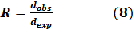
The ratio is less than 1 if the point pattern is more clustered than random and greater than 1 if the point pattern is more dispersed than random. Nearest Neighbor analysis can also produce a score, which indicates the likelihood that the pat- tern could be a result of random chance [1] [21] [33].

(a) (b)
Figure 3.5 (a) shows the Crime Incidents and (b) shows the
Natural Neighbor opertation on (a)
The Fig. 3.5 (a) shows the crime events and (b) shows the Hot Spot identified by applying Natural Neighbor operation. The circle shows the detected Hot Spot.

International Journal of Scientific & Engineering Research, Volume 5, Issue 12, December-2014 1334

ISSN 2229-5518

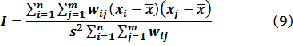
3.6 Moran’s I for Measuring Spatial Autocorrelation

Nearest neighbor analysis requires only the distances between points as inputs for the calculation. Analysis of Spatial Auto- correlation on the other hand considers both the point loca- tions and the variation of an attribute at the locations. Spatial Autocorrelation therefore measures the relationship among values of a variable according to the spatial arrangement of the values. The relationship may be describes as highly corre- lated if like values are spatially close to each other and inde- pendent or random if no pattern can be discerned from the arrangement of values [15]. Moran’s I can be computed by using the following formula:

where is the value at point is the value at point is a coefficient, is the number of points, and is the variance of values with a mean of . The coefficient is defined as the inverse of the distance ( ) between points and or 1/ . Other weights such as the inverse of the distance
squared can also be used [1].

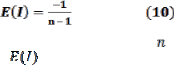
The values Moran’s I takes on are anchored at the ex- pected values for a random pattern:
approaches 0 when the number of points is large. Moran’s I is close to if the pattern is random. It is greater than if adjacent points tend to have similar values (i.e. are spatially correlated) and less than if adjacent points tend to have different values (i.e. are not spatially correlated).
Similar to nearest neighbor analysis, the Z score associated with a Moran’s I can be computed. The Z score indicates the likelihood that the point pattern could be a result of random chance [34].

Moran’s I can also be applied to area patterns. Eq. 10 re- mains the same for computing the index value. The difference is the coefficient which is now based on the spatial rela- tionship between polygons. One option is to assign 1 to if polygon is adjacent to polygon and 0 if and are not adja-

cent to each other [1] [20] [22] [35].

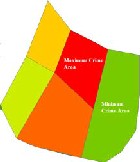
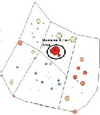
(a) (b)
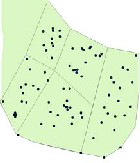
Figure 3.6 (a) shows Maximum Crime Zone (point feature)
(b) shows Maximum Crime Area using Moran’s I operation
The Fig. 3.6 (a) shows the Moran’s-I operation on Point feature with the circle showing the identified Maximum Crime Area. (b) Shows the Moran’s-I operation on Polygon feature with the Maximum and Minimum Crime Area identified.

3.7 G-Statistics for Measuring High/Low Clustering

Moran’s I either general or local can only detect the presence of the clustering of similar values. It cannot indicate whether the clustering is made of high values or low values. This led to the use of the G-statistics, which can separate clusters of high values from clusters of low values [36]. The general G- statistics based on a specified distance is defined as:

where is the value at location , is the value at loca- tion if is within of , and is the spatial weight. The weight can be based on some weighted distance (e.g. inverse distance) [1].

The expected value of is:

is typically a very small value when is large.

A high value suggests a clustering of high values and a low value suggests a clustering of low values. Z score can be computed for a to evaluate its statisti-
cal significance. The local G-statistics denoted by is
often described as a tool for “Hotspot” analysis. A cluster
of high positive Z scores suggests the presence of a cluster

of high values or a hot spot. A cluster of high negative Z scores, on the other hand suggests the presence of a cluster of low values or a cold spot. The local G-statistics also al- lows the use of a distance threshold , defined as the dis- tance beyond which no discernible increase in clustering of high or low values exists [1] [22] [33].

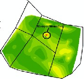
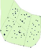
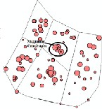
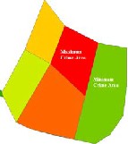
(a) (b)
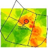
Figure 3.7 (a) shows the Maximum Crime Zone (point
feature) and (b) shows the Maximum Crime Area
(polygon feature) using Getis-Ord Gi* operation
The Fig. 3.7 (a) shows the Getis-Ord Gi* operation on Point feature with the circle showing the identified Maximum Crime Area. (b) shows the Gi* operation on Polygon feature

International Journal of Scientific & Engineering Research, Volume 5, Issue 12, December-2014 1335

ISSN 2229-5518

with the dark Red area showing Maximum and dark Green area showing Minimum Crime Area identified.

4 DISCUSSION ON THE METHODS

The following tables shows different methods discussed so far, Table 4.1 discusses the Formula and the Purpose of the methods for Hot Spot Analysis. Table 4.2 shows the features on which the methods can be applied, it also discuss about how the output of the methods will be displayed like smooth- ing effect and also the additional variable like Z-score calcu- lated by some methods.

Table 4.1 Different Methods for Crime Analysis
Table 4.2 Usefulness of the Methods

5 CONCLUSION

Crime Mapping and Analysis can effectively provide the un- derstanding of where and why crime activity takes place and by using this information Law enforcement agencies can take appropriate action in very efficient and effective manner. Dif- ferent methods are classified based on the input feature and the input parameters. The methods can also be used as per the requirement of the problem. KDE and Thin-plate Spline pro-
vide the smoothing surface, while IDW can be used when we require having a specific range of maximum and minimum values. Moran’s I can be used for both point and polygon fea- tures and can detect the presence of the clustering of similar values, whereas Getis-Ord Gi* can separate the clusters of high and low values and can be applied for point and polygon features. The Moran’s I and Gi* both also calculate the value
for the analysis purpose.

ACKNOWLEDGEMENT

Authors would like to acknowledge and extend heartfelt grat- itude to UGC (University Grant Commission) for develop- ment of Geospatial Technology Laboratory to complete this work under UGC SAP (II) DRS Phase-I F. No.-3-42/2009 and One Time Research Grant F. No. 4-10/2010 (BSR) to Depart- ment of Computer Science and IT, Dr. Babasaheb Ambedkar Marathwada University, Aurangabad, M.S., India.

REFERENCES

[1] Kan-tsung Chang; Introduction to Geographic Information Sys- tem (4th Edition, Tata McGraw-Hill, Eleventh Reprint 2012).

[2] Rachel Boba; Crime Analysis and Crime Mapping (Sage Publi-

cations, Inc., printed in United States of America, 2005).

[3] Nagne Ajay D., Amol D. Vibhute, Bharti W. Gawali, and Suresh C. Mehrotra; Spatial Analysis of Transportation Net- work for Town Planning of Aurangabad City by using Geographic Information System; IJSER, 2013.

[4] Nagne Ajay D., and Bharti W. Gawali; Transportation network analysis by using Remote Sensing and GIS a Review; IJERA,

2013.

[5] S. S. Khadilkar, S. M. Ansari, S. S. Raut, and A. S. Gaikwad;

Detection of Reliable Route in Transportation Network Using

GIS: A Review; IJERT, 2014.

[6] Francis Fajemirokun, O. Adewale, Timothy Idowu, Abimbo- la Oyewusi and Babajide Maiyegun; A Gis Approach To Crime Mapping And Management In Nigeria: A Case Study Of Victoria Island Lagos; Shaping The Change xxiii Fig Congress Munich, Germany, 2006.

[7] M. Ahmed and R. S. Salihu; Spatiotemporal Pattern of Crime

Using Geographic Information System (GIS) Approach in Dala

L.G.A of Kano State, Nigeria; AJER, 2013.

[8] Keith Harries; Mapping Crime Principle and Practice (U.S. De- partment of Justice Programs, National Institute of Justice; Washington, DC 20531, December 1999).

[9] Guta R., Rajitha K., Basu S. and Mittal S.; Application of GIS

in Crime Analysis: A Gateway to Safe City, India Geospatial Fo- rum, 2012.

[10] Christopher W. Bruce; Fundamentals of Crime Analysis (Chap- ter 1, Exploring Crime Analysis, 2nd Edition, IACA, Over- land Park, KS, http://iaca.net/ExploringCA/exploringca

_chapter1.pdf, accessed on 23-04-2014).

[11] Lauren Scott and Nathan Warmerdam, Extend Crime Anal- ysis with ArcGIS Spatial Statistics Tools (www.esri.com/news/rcuser/0405/ss_crimestat1of2.htm l, accessed on 20-04-2014).

International Journal of Scientific & Engineering Research, Volume 5, Issue 12, December-2014 1336

ISSN 2229-5518

[12] Liu Lei, The GIS-based Research on Criminal Cases Hotspots

Identifying, ICESE, 2011.

[13] Jitendra Kumar, Sripati Mishra and Neeraj Tiwari; Identifi- cation of Hotspots and Safe ones of Crime in Uttar Pradesh, India: Geo-spatial Analysis Approach; IJRSA, 2012.

[14] http://resources.arcgis.com/en/help/main/10.1/002t/0
02t0000000z000000.htm; accessed on 2-12-2013.

[15] http://support.esri.com/en/knowledgebase/Gisdictionary

/browse; accessed on 29-04-2014.

[16] Xiao Qin, Steven Parker, Yi Liu, Andrew J. Graettinger and Susie Forde; Intelligent geocoding system to locate traffic crashes, Accident Analysis and Prevention, Elsevier, 2013.

[17] M. Vijaya Kumar and Dr. C. Charasekar; Spatial Statistical

Analysis of burglary Crime in Chennai City Promoters

Apartments: A Case Study, IJETT, 2011.

[18] http://www.gisresources.com/types-interpolation-

methods_3/; accessed on 29-04-2014.

[19] Giles C. Oatley and Brian W. Ewart; Crimes analysis soft-

ware: ‘pins in maps’, clustering and Bayes net prediction; Expert System with Applications, Pergamon, 2003.

[20] Dr. M. VijayaKumar, Dr. S. Karthick and N.Prakash; The

Day-To-Day Crime Forecasting Analysis Of Using Spatial- Temporal Clustering Simulation; IJSER, 2013.

[21] S. R. Sathyaraj, A. Thangavelu, S. Balasubramanian, R. Sri- dhar, M.Chandran and M. Prashanthi Devi; GIS Analysis of Spatially-Referenced Auto Vehicle Theft Crime In Coimba- tore Urban, India: Visualization Through Kernel Estimation;

3rd International Conference On Cartography And GIS, 15-

20 June, 2010.

[22] V. Prasannakumar, H. Vijith, R. Charutha and N. Geetha; Spatio-Temporal Clustering Of Road Accidents: GIS Based Analysis And Assessment; International Conference: Spatial Thinking and Geographic Information Sciences, Elsevier,

2011.

[23] GiedrėBeconytė, AgnėEismontaitė and Denis Romanovas; Analytical mapping of registered criminal activities in Vil- nius city; Geodesy and Cartography, 2012.

[24] Katie Lyon, Stuart P. Cottrell, Pirkko Siikamaki and Ramona

Van Marwijk; Biodiversity Hotspots And Visitor Flows In Oulanka National Park, Finland; Journal of Hospitality and Tourism, Taylor & Francis, 2011.

[25] M.Vijaya Kumar and C.Chandrasekar; GIS Technologies in

Crime Analysis and Crime Mapping; IJSCE, 2011.

[26] http://resources.arcgis.com/en/help/main/10.1/index.ht ml#/How_Kriging_works/; accessed on 04-12-2013.

[27] George Grekousis and Yorgos N. Photis; Analyzing High-

Risk Emergency Areas with GIS and Neural Networks: The

Case of Athens, Greece; The Professional Geographer, 2013.

[28] HarsihKumar R and Sujatha R; A Framework for Detecting

Hotspots Using Clustering; Paripex- IJR, 2013.

[29] C.P. Johnson; Crime Mapping and Analysis Using GIS; Ge-

omatics 2000, Conference on Geomatics in Electronic Gov- ernance, 2000.

[30] Sangamithra. V, T. Kalaikumaran and Dr. S. Karthik; Data mining techniques for detecting the crime hotspot by using GIS; IJARCET, 2012.

[31] Esri, Inc., GIS Provides the Geographic Advantages- for In- telligence-Led policing,

www.esri.com/lawenforce; accessed on 7-12-2013.

[32] Tony H. Grbesic and Alan T. Murray; Detecting Hot Spots using Cluster Analysis and GIS; Proceedings from the Fifth Annual International Crime Mapping Research Confer- ence. Dallas, TX, 2001.

[33] Weimin Li and john D. Radke; Geospatial data integration and modeling for the investigation of urban neighborhood crime; Annals of GIS, 2012.

[34] Christopher Fulcher and Catherine Kaukinen PhD; Mapping and visualizing the location HIV service providers: An ex- ploratory spatial analysis of Toronto neighborhoods; AIDS Care: Psychological and Socio-medical Aspects of AIDS/HIV, 2005.

[35] Jane L. Garb and Richard B. Wait; Using Spatial Analysis To Improve Health Care Services And Delivery At Baystate- Health; Journal of Map & Geog. Libraries: Advances in Geo- spatial Information, Collection & Archives, Taylor & Fran- cis, 2011.

[36] Fahui Wang; Why Police and Policing need GIS: An Over- view; Annals of GIS, 2012.