International Journal of Scientific & Engineering Research, Volume 5, Issue 3, March-2014 1103

ISSN 2229-5518

Medical Image Compression using iterated graph cuts based segmentation and modified fast SPIHT encoding

S.Jagadeesh1, Dr.E.Nagabhooshanam2

1(Assoc. Prof. & Head of the Department, Electronics and Communications Engineering Department, SSJ Engineering College/ JNTU, Hyderabad, Andhra Pradesh, India)

2(Dr. Prof. & Head of the Department, Electronics and Communications Engineering Department, Sridevi Women’s Engineering

College/ JNTU, Hyderabad, Andhra Pradesh, India)

Abstract— In diagnostic MRI, it is routine to acquire multiple images of the same region of interest (ROI) with different segments. In such segments acquisition, joint Level Set Segmentation exploits the mutual information across the shared ROI for improved image quality in accelerated acquisitions with under sampling of each contrast. Transmission of such segments by encoding through lossy channel was implemented in SPIHT. The above methods having more redundancy bits and more reconstruction time during the implementation. To improve the segmentation and compression time, we are proposing modified fast SPIHT (MFSPIHT) encoding technique where interactive graph cut based segmented image is compressed using MFSPIHT and recovered in both loss less and lossy transmission mediums. Proposed method has shown better comparative results.

Index Terms—MRI, region of interest, Level Set Segmentation, SPIHT, interactive graph cut based segmentation.

——————————  ——————————

1 INTRODUCTION

MAGE segmentation is an essential tool in medical image processing and is used in various applications. For example, in medical imaging filed is used to detect multiple sclerosis
lesions quantification, surgical planning, conduct surgery simulations, locate tumors and other pathologies, measure tissue volumes, brain MRI segmentation, study of anatomical structure etc. Other practical applications of image segmenta- tion are machine vision, traffic control system; face and finger print recognition and locate objects in satellite images. Image segmentation with graph cuts technique has potential useful- ness for everyday applications like image cropping and colori- zation along with the multi-view image stitching, video tex- ture synthesis, image reconstruction, n-dimensional image segmentation etc.
Graph-cuts are one of the leading segmentation techniques to efficiently solve a wide variety of brain tissue identification. Energy minimization along with image smoothing is per- formed with the graph cuts method. Different types of algo- rithms such as new minimum-cut/maximum flow (min- cut/max-flow), push-relabel, augmenting paths etc. are used in graph cuts method as well as the normalized cut.
Medical images contain information critical to accurate diag- nosis. As a consequence of this, it is desirable that any com- pression operation performed on medical images should not remove vital diagnostic information. The current preferred method for compressing medical images is through lossless coding. The current standardized lossless coders for medical imaging include JPEG lossless compression [1], the JPEG-LS compression [3] and the lossless mode of the proposed JPEG
2000 scheme [5]. The performance evaluation of different loss- less medical image compression methods and their effects have been summarized in [7]. The Digital Imaging and Com- munication in Medicine (DICOM) [6] standard supports both the JPEG and the JPEG 2000 compression scheme. In lossy
compression, the deterioration of information may lead to mis-diagnosis. However, it is possible to allow controlled deg- radation of information without impeding the diagnostic in- formation in medical images. Such an approach may be found in the SPIHT.

2. EXISTING METHODS

2.1 A Variational Level Set Approach to Segmentation Consider the case of N=2. In this case, the image domain is partitioned into two regions {Ωi}2 i=1 . These two regions can be
represented by the regions separated by the zero level contour
of a function φ, i.e.,Ω1={φ>0}andΩ2={φ<0}.Using Heaviside
function H, the energy E Eq. (1) & (2) can be expressed as an
energy in terms of φ, b,and c as below

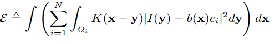
…Eqn. (1)

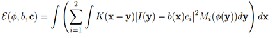
….Eqn. (2)
Where M1(φ(x)) = H(φ(x)) and M2(φ(x)) = 1−H(φ(x)). In prac- tice, a smoothed Heaviside function Hε (x)= ½[1+2/π arctan(x/ε)] to approximate the original Heaviside function H, with ε=1. It is necessary to add a regularization term R(φ)to the above energy in the following energy functional:

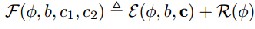
…Eqn. (3)

IJSER © 2014 http://www.ijser.org

International Journal of Scientific & Engineering Research, Volume 5, Issue 3, March-2014 1104

ISSN 2229-5518

The first term in R serves to regularize the zero level contour of φ as in typical level set methods, while the second term regularizes the entire level set function φ by penalizing its de- viation from signed distance, as in the level set methods pro- posed by Liet al. The energy ε(φ,b,c) is the data term in varia- tional framework. Similarly, multiple level set functions φ1,···,φn to represent regions {Ωi}Ni=1 with N=2n as in [4]. For
convenience, a vector valued function Φ=(φ1,···,φn) to repre-
sent the functions φ1,···,φn. The energy for general multiphase
formulation of our method can be defined as

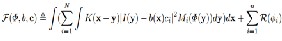…Eqn. (4)

Where Mi(Φ) are functions of Φ which are designed such that ΣNi=1 Mi(Φ)=1.The definition of Mi in the four-phase case are given. For N=3 and two level set functions φ1 and φ2, M1(φ1,φ2)=H(φ1)H(φ2), M2(φ1,φ2)= H(φ1)(1−H(φ2)),andM3(φ1,φ2)=1−H(φ1)to obtain a three- phase formulation.
For fixed c and b, the minimization of F(φ,c,b) consists in solv- ing the level set evolution equation as the gradient
Fig 1 (a): Image with seeds. Fig 1 (d): Segmentation results.

…Eqn. (5)
Where ∂F/∂φ is the Gӑteaux derivative (the first order func- tional derivative) of the energy F. In numerical implementa-
Fig 1 (c): Cut.

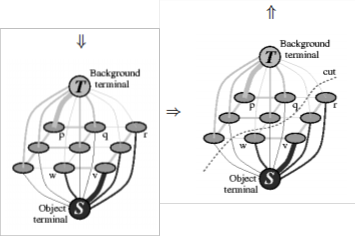
Fig 1 (b): Graph.

tion, at each iteration according to Eq. (9), the variables c and b are updated according to the following procedure. For fixed φ and c, an optimal bias field b that minimizes F(φ,c,b). It can be shown that the minimize b is
…Eqn. (6)
Where ∗ is the convolution operation, and J (1)=ΣN i=1 ci Mi (φ)
and J(2) =ΣN i=1 c2 i Mi (φ). For fixed φ and b, an optimal c that
minimizes F(φ,c,b). By some calculus manipulations, it can be shown that the minimize c=(ci ,···,cN ) is

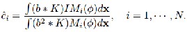…Eqn. (7)

It is worth noting that the expression of b in Eq. (10) with con- volutions shows that b is smooth. The smoothness of b is in- trinsically ensured by the data term E(φ,c,b) in variational framework. This is a desirable advantage of this method: there is no need for imposing a smoothing term to ensure the smoothness of the bias field.

2.2 Interactive Graph Cuts Based Segmentationg

This technique is based on powerful graph cut algorithms from combinatorial optimization. Implementation uses a new version of “max-flow” algorithm.
Figure 1. A simple 2D segmentation example for a 3 × 3 image. The seeds are O = {v} and B = {p}. The cost of each edge is re- flected by the edge’s thickness. The regional term (2) and hard constraints (4,5) define the costs of t-links. The boundary term (3) defines the costs of n-links. Inexpensive edges are attractive choices for the minimum cost cut. Assume that O and B de- note the subsets of pixels marked as “object” and “back-
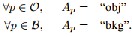
ground” seeds. Naturally, the subsets O ⊂ P and B ⊂ P are
such that O ∩ B = ∅. Remember that to compute the global
minimum of (1) among all segmentations A satisfying hard
constraints

….Eqn. (8) The general work flow is shown in Figure 1. Given an image (Figure 1(a)) we create a graph with two terminals (Figure

1(b)). The edge weights reflect the parameters in the regional (2) and the boundary (3) terms of the cost function, as well as the known positions of seeds in the image. The next step is to compute the globally optimal minimum cut (Figure 1(c)) sepa- rating two terminals. This cut gives segmentation (Figure 1(d)) of the original image. In the simplistic example of Figure 1 the image is divided into exactly one “object” and one “back- ground” regions. To segment a given image a graph G = hV ,
Ei with nodes corresponding to pixels p ∈ P of the image.
There are two additional nodes: an “object” terminal (a source
S) and a “background” terminal (a sink T ). Therefore

IJSER © 2014 http://www.ijser.org

International Journal of Scientific & Engineering Research, Volume 5, Issue 3, March-2014 1105

ISSN 2229-5518

V = P {S, T}.
2.3 Set Partitioning In Hierarchical Trees (SPIHT)
SPIHT is the wavelet based image compression method. It
provides the Highest Image Quality, Progressive image
transmission, fully embedded coded file, Simple quantiza-
tion algorithm, fast coding/decoding, completely adaptive,
Lossless compression, Exact bit rate coding and Error pro- tection. SPIHT makes use of three lists – the List of Significant Pixels (LSP), List of Insignificant Pixels (LIP) and List of Insig- nificant Sets (LIS). These are coefficient location lists that con-
tain their coordinates. After the initialization, the algorithm takes two stages for each level of threshold – the sorting pass (in which lists are organized) and the refinement pass (which does the actual progressive coding transmission). The result is in the form of a bit stream. It is capable of recovering the im- age perfectly (every single bit of it) by coding all bits of the transform. However, the wavelet transform yields perfect reconstruction only if its numbers are stored as infinite impre- cision numbers.

3 PROPOSED METHOD OF IMAGE COMPRESSION

In our proposed method, we had taken modified graph cuts algorithm and modified fast improved SPIHT. In the original graph cuts algorithm, the segmentation is directly performed on the image pixels. There are two problems for such a pro- cessing. First, each pixel will be a node in the graph so that the computational cost will be very high; second, the segmenta- tion result may not be smooth, especially along the edges. These problems can be solved by introducing some low level image segmentation techniques, such as watershed and mean shift, to graph cuts. We choose to use mean shift for initial segmentation because it produces less over-segmentation and has better edge preservation.
Wavelet transform image coding using SPIHT Traditional
SPIHT has the advantages of embedded code stream structure, high compression rate, low complexity and easy to implement. Improved SPIHT algorithm mainly makes the fol- lowing changes.
• SPIHT codes four coefficients and then shifts to the next four ones.
• When computing the maximum threshold, the im- proved algorithm can initialize the maximum of every block.
• The coefficients in non-important block will be coded in next scanning process or later, rather than be coded in the present scanning process .
• Our algorithm encodes the sub band pixels by performing initialization and a sequence of sorting pass, refinement pass and quantization-step updat- ing. However, differences of initialization and sorting pass still exist between the improved SPIHT [3] and traditional SPIHT.

3.1 FLOW CHART OF PROPOSED METHOD

We had taken MR images for our method implementation,
• Step 01: Read input image; convert that image in to
gray image.
• Step 02: Apply that image to segmentation process.
• Step 03: Extract the segmented image.
• Step 04: Compress the extracted image using
MFSPIHT.
• Step 05: Extract the compressed image.
• Step 06: Perform inverse MFSPIHT
• Step 07: Reconstruct the original image.
Patient’s data which we had taken for analysis are tabulated in
table 1.
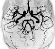
Table 1 Patient’s data.

IJSER © 2014 http://www.ijser.org

International Journal of Scientific & Engineering Research, Volume 5, Issue 3, March-2014 1106

ISSN 2229-5518

4 Results and Discussions

We had compared our proposed method with
1. Set Partitioning in Hierarchical Trees (SPIHT)
2. A Variational Level Set Approach to Segmentation
(VLSAS)
3. Interactive Graph Cuts based segmentation (IGCS)
4. VLSAS through SPIHT (VLSSPIHT)
5. IGCS through SPIHT (IGCSSPIHT)-Our proposed
method
Comparative results for Patient 01 Image tabulated in Table 2.
Table 2 Comparative Results: Patient 01

IJSER © 2014 http://www.ijser.org

International Journal of Scientific & Engineering Research, Volume 5, Issue 3, March-2014 1107

ISSN 2229-5518

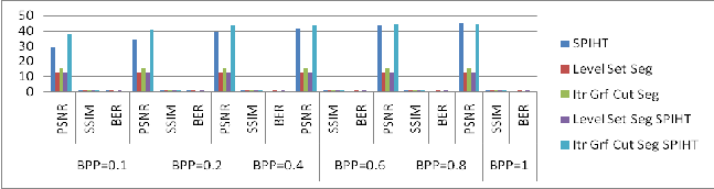
Figure 2: Comparative Results: Patient 01with different BPP values.
Comparative results for Patient 01 Image, Patient 02 Image, Patient 03 Image and Patient 04 Image tabulated in Table 3.
Table 3 Comparative Results: Patient 01, Patient 02, Patient 03 and Patient 04 with BPP=0.6.

IJSER © 2014 http://www.ijser.org

International Journal of Scientific & Engineering Research, Volume 5, Issue 3, March-2014 1108

ISSN 2229-5518

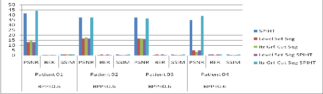
Figure 3: Comparative Results: Patient 01, Patient 02, Patient 03 and Patient 04 with different BPP=0.6 values.
From the above comparative results, using our method a segmented image can be compressed. Compressed image can be reconstructed with minimum 50 % accuracy.

5 Conclusions

Our proposed modified Interactive Graph Cuts based segmen- tation (IGCS) algorithm can be applicable to low resolution MR images; segmented image shows better segmentation comparatively. And modified fast Set Partitioning in Hierar- chical Trees (SPIHT) had shown better results for high com- pression. Our proposed algorithm had shown better results by combining low resolution segmentation and high compres- sion. An efficient segmented compression technique for MR Images is proposed in our algorithm.

6 Future Research

Our proposed method can be further applicable to improve the memory size of compressed image. CT images and DI- COM Images can also be compressed using our proposed al- gorithm. Using our method, hardware implementation for proposed algorithm becomes flexible and easy. Further our
proposed algorithm can be applicable to high speed image decoding techniques where high scalable images are required.

REFERENCES

[1] Wells, W., Grimson, E., Kikinis, R., Jolesz, F.: Adaptive segmentation of

MRI data. IEEE Trans. Med. Image. 15(4), 429–442 (1996)

[2] Vovk, U., Pernus, F., Likar, B.: A review of methods for correction of in- tensity in homogeneity in mri. IEEE Trans. Med. Image. 26(3), 405–421 (2007)

[3] Lewis, E., Fox, N.: Correction of differential intensity in homogeneity in longitudinal MR images. Neuro image 23(3), 75–83 (2004)

[4] Dawant, B., Zijdenbos, A., Margolin, R.: Correction of intensity varia- tions in MR images for computer-aided tissues classification. IEEE Trans. Med. Image. 12(4), 770–781 (1993)

[5] Meyer, C., Bland, P., Pipe, J.: Retrospective correction of intensity in ho- mogeneities in MRI. IEEE Trans. Med. Image. 14(1), 36 (1995)

[6] Sled, J., Zijdenbos, A., Evans, A.: A nonparametric method for automatic correction of intensity no uniformity in MRI data. IEEE Trans. Med. Imag- ing 17(1), 87–97 (1998)

[7] Leemput, K., Maes, F., Vandermeulen, D., Suetens, P.: Automated mod- el-based bias field correction of MR images of the brain. IEEE Trans. Med. Image. 18(10), 885–896 (1999)

IJSER © 2014 http://www.ijser.org

International Journal of Scientific & Engineering Research, Volume 5, Issue 3, March-2014

ISSN 2229-5518

1109

IJSER lb)2014

http://www.ijserorq