International Journal of Scientific & Engineering Research,Volume 3, Issue 9, September-2012 1
ISSN 2229-5518
Mathematical Time Domain Study of Negative
Feedback System Using Limiting Progression
Arindam Bose
Abstract—Every stable feedback system has certain finite limiting value with respect to time. This paper describes a mathematical analytical study for stable negative feedback system with the help of limiting progressions. Some limiting progressions descr ibed in this paper have a finite limiting value which can be predicted previously using the characteristics parameters of the system by analytical method. Some of these parameters are independent and primary properties of the system itself. The final value of the feedback system having transfer function as a limiting progression can be predict ed and sometimes be controlled using the parametric solution.
Index Terms—Control system, Limiting progression, Limiting progressive function, Negative feedback system, Predicting expression, Transfer function.
1 INTRODUCTION
————————————————————
OSTof the negative feedback systems are stable with respect to time, as they converge to a finite limiting val- ue. And marginally stable feedback systems are
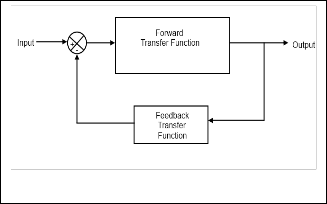
bounded-oscillatory in nature.Fig.1 describes a general confi- guration a negative feedback system.
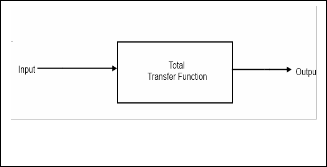
Fig.1.a. General Representation of Negative Feedback System
Fig.1.b. Equivalent Representation of Negative Feedback Sys- tem
We know that every negative feedback system has a damp- ing coefficient (ζ) depending which they are classified into three sections:
————————————————
 Arindam Bose is currently pursuing BTech degree program in electronics and communication engineering from Future Institute of Engineering and Management of West Bengal University of technology, India, PH -
+919051320505. E-mail: adambose1990@gmail.com
a. Under-damped system,
b. Critically damped system and
c. Over-damped system.
Now in this paper we will discuss about the mathematical
study of these three systems with the help of Limiting Pro-
gressions.
Definition of Limiting Progressions: There are some sorts of
series which are defined by a single valued iterative function
(expression), where the result (dependent variable) is again
used as the independent variable in the same expression and a
limiting value can be reached as we go for infinite times of
iteration. This type of series can be called as LIMITING PRO- GRESSION. So, in Limiting Progression the output is totally feedback to the input, NOT partially. Rather we can say that the output in certain state is totally put as the input of the next
state.

i.e. if  is the iterative function of random variable


and  be the order of iteration and is defined as


 and
and  (constant), then is
called LIMITING PROGRESSIVE FUNCTION.
And the equation  which predicts

this constant term is called PREDICTING EXPRESSION.

Such that 
2 DISCUSSION ABOUT SOME TYPES OF LIMITING
PROGRESSIONS
Let us consider some types of limiting progressions.
2.1 Type I
Limiting Progressive Function:


Where  represents set of REAL numbers and I represents set of INTEGERS.


Predicting Expression:  Form:
Form:

IJSER © 2012
http://www.ijser.org
where  is a random variable,
International Journal of Scientific & Engineering ResearchVolume 3, Issue 9, September-2012 2
ISSN 2229-5518


is a real constant, is a real constant,
isthe order of iteration. … (1.1)
This is one of the limiting series. Here we begin with  as a
as a
random variable, then apply to (1.1). We get a result. This re-
sult is now treated as  . So further repeating this iterative
method, we will be getting a limiting value where


 (constant).
This series is an infinite series. But it has a limiting value
towards the end. We can get the limiting value by considering
the expression:

 … (1.2)


So (1.2) does not depend on , rather depends on  and . Now take an example:

Ex. 1.1: Suppose we take a random set, such as  ,
, 
 and
and  .
.


So 


 for
for

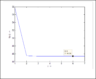
From the expression(1.2) you can previously predict the limit- ing value of the series, which will be 


Now if you take 9 digits after decimal point, the series will be:

6·000000544 for 


6·000000272 for 


6·000000136 for 


6·000000068 for 


6·000000034 for 


6·000000017 for 


6·000000008 for 


6·000000004 for 

6·000000002 for 

6·000000001 for 

6·000000001 for 

6·000000000 for 

6·000000000 for 

… value repeating
or approx. 6.


 and so on. Next results will be:
151·9375 for 


78·96875 for 


42·484375 for 


24·2421875 for 

15·12109375 for 

10·56054688 for 


8·280273438 for 


7·140136719 for 


6·570068359 for 


6·28503418 for 


6·14251709 for 


6·071258545 for 


6·035629272 for 


6·017814636 for 


6·008907318 for 


6·004453659 for 

6·00222683 for 

6·001113415 for 

6·000556707 for 

6·000278354 for 

6·000139177 for 

6·000069588 for 

6·000034794 for 

6·000017397 for 

6·000008699 for 

6·000004349 for 


6·000002175 for 


6·000001087 for 

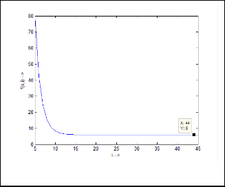
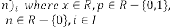
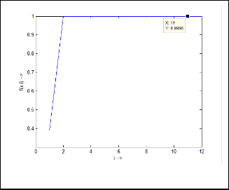
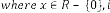
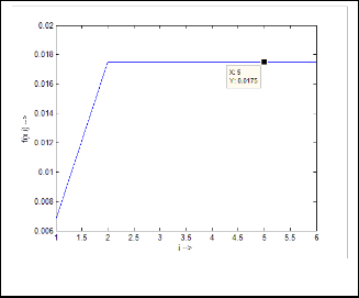
Fig.2.a. Output response of Ex.1.1
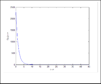
Fig.2.b. More detailed and zoomed in output response of Ex.1.1
So (1.2) is true analytically.

Ex.1.2: Now take another set for example for  ,
,


, 
 and
and  and put them into (1.1)

Here also our predicted result will be  , as seen earlier.
IJSER © 2012
http://www.ijser.org
International Journal of Scientific & Engineering ResearchVolume 3, Issue 9, September-2012 3
ISSN 2229-5518
So the results will be:


 for
for 

Next iterative results will be:
35·3225 for 


20·66125 for 

13·330625 for 


9·6653125 for 


7·83265625 for 


6·916328125 for 

6·458164063 for 

6·229082031 for 


6·114541016 for 


6·057270508 for 


6·028635254 for 


6·014317627 for 


6·007158813 for 


6·003579407 for 


6·001789703 for 


6·000894852 for 


6·000447426 for 


6·000223713 for 

6·000111856 for 

6·000055928 for 

6·000027964 for 

6·000013982 for 

6·000006991 for 

6·000003496 for 

6·000001748 for 

6·000000874 for 

6·000000437 for 

6·000000218 for 


6·000000109 for 


6·000000055 for 


6·000000027 for 


6·000000014 for 


6·000000007 for 


6·000000003 for 


6·000000002 for 


6·000000001 for 


6·000000000 for 


6·000000000 for 

…value repeating
or approx. 6.
Fig.3. Output response of Ex.1.2

So (1.2) is true analytically whatever may be. Ex.1.3: Now we take another example:


 for
for
The prediction for answer is: 
Now let’s see, 

The iterative results are:

57·58677686 for 

45·47592378 for 


45·37583408 for 

45·37500689 for 


45·37500006 for 


45·375 for 


45·375 for 

…value repeating
Fig.4. Output response of Ex.1.3
IJSER © 2012
http://www.ijser.org
International Journal of Scientific & Engineering ResearchVolume 3, Issue 9, September-2012 4
ISSN 2229-5518
Ex.1.4: Now we are taking another different example:


for 


for 


for

Predicted answer is: 
Now let’s see, 
The iterative results are:

–15·96526316 for 

–5·159722992 for 


–5·728435632 for 

–5·698503388 for 


–5·700078769 for 


–5·699995854 for 


–5·700000218 for 

–5·699999989 for 

–5·700000001 for 


–5·7 for 


–5·7 for 

… value repeating


for  and so on…


Here is not allowed as the term  is not allowed. So, for
  be the iterative function of random variable

and  be the order of iteration and is defined as


 , then
 constant.
So this is an example of limiting progression.
2.2 Type II
Limiting Progressive Function:


Predicting Expression:


Form:


 where
where  is a random variable,
Fig.5. Output response of Ex.1.4
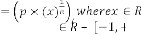
Then our prediction was right and exact in all the cases. Some limiting values for real variable p :
Take p be 1,2,3 and so on and n be another real variable. Then the results will be:


for  [‘ ’ indicates the limiting value]


for  for
for


is a real constant,
 is a real constant,
is the order of iteration. … (2.1)

Here also we begin with as a random variable, then apply it
to (2.1). We get a value of  . This result now will be

treated as next . Further we are going to apply it to (2.1) and
so on and so forth.
This series also has no end; rather it has a limiting value. We can get the limiting value by considering the following expres- sion:

 … (2.2)


So (2.2) does not depend on , rather depends on  and and sign of .
Let’s consider different cases:
Case (1): 


In this case the limiting value will be:


for  for
for  for
for

Let’s take some examples.


Ex.2.1: Initialize 
 for
for
IJSER © 2012
http://www.ijser.org
… (2.3)
International Journal of Scientific & Engineering ResearchVolume 3, Issue 9, September-2012 5
ISSN 2229-5518
So predicted answer is:
Now let’s calculate  for different values of
  . The iterative results will be:


5·68773396
3·570067442
3·056718667
2·902564095
2·852926624
2·836570158
2·831138868
2·829330751
2·828728301
2·828527513
2·828460587
2·828438279
2·828430843
2·828428364
2·828427538
2·828427262
2·828427171
2·82842714
2·82842713
2·828427126
2·828427125
2·828427125
…value repeating
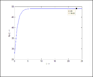
Now let’s calculate  for different values of
  . The iterative results will be:


40·08891269
45·74210241
47·87093724
48·62776152
48·89150021
48·98277586
49·01428972
49·02516127
49·02891064
49·03020359
49·03064944
49·03080319
49·0308562
49·03087448
49·03088079
49·03088296
49·03088371
49·03088397
49·03088406
49·03088409
49·0308841
49·0308841
…value repeating
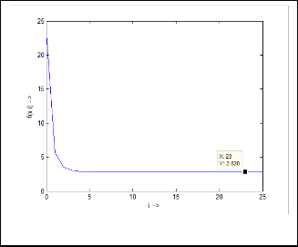
Fig.7. Output response of Ex.2.2
So (2.3) is proved analytically.
Fig.6. Output response of Ex.2.1
So (2.3) is proved analytically.

If we take 


Here also the limiting value will be 2·828427125  .
.

Case (2): 
 In this case the limiting value will be:
… (2.4)


So (2.3) is true always for a single set of  .
.
Ex.2.2: Now let’s take another example:


Take =27·345,  =12·81, =2·9


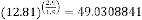
Our predicted answer will be:

Ex.2.3: Take an example: 

 (odd tak- en).
Now the expression will be:


IJSER © 2012
http://www.ijser.org
International Journal of Scientific & Engineering ResearchVolume 3, Issue 9, September-2012 6
ISSN 2229-5518


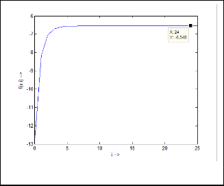
Predicted answer: 
The iterative results will be:


–8·159438048
–7·04619721
–6·709955537
–6·601479188
–6·565711522
–6·553832083
–6·549877049
–6·548559235
–6·548120022
–6·547973624
–6·547924826
–6·54790856
–6·547903138
–6·54790133
–6·547900728
–6·547900527
–6·54790046
–6·547900438
–6·547900431
–6·547900428
–6·547900427
–6·547900427
…value repeating
In this case the positive and negative limiting values will gradually come one after one and the system will be oscillato- ry.

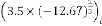
Ex.2.5: Take an example: 
 Predicted answer is:


Now the iterative results for will be as follows:
–2·5198421
2·72158
–2·792353286
2·816351026
–2·824396016
2·827082783
–2·82797894
2·828277722
–2·828377323
2·828410524
–2·828421591
2·82842528
–2·82842651
2·82842692
–2·828427056
2·828427102
–2·828427117
2·828427122
–2·828427124
2·828427124
–2·828427125
2·828427125
–2·828427125
2·828427125
…value repeating
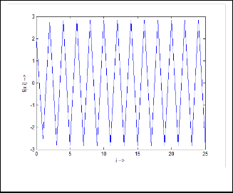
Fig.8. Output response of Ex.2.3
So (2.4) is proved analytically.

Ex.2.4: Take another example: 
 (even taken).
So the expression will be:
is not defined.

Case (3):  ,
, 
Here the limiting value should be:


… (2.5)
Fig.9. Output response of Ex.2.5
So (2.4) is proved analytically.
IJSER © 2012
http://www.ijser.org
International Journal of Scientific & Engineering ResearchVolume 3, Issue 9, September-2012 7
ISSN 2229-5518
Case (4): 
In this case the predicted answer will be as (2·3) i.e.


Ex.2.6: Example: 
 Predicted answer:
But in case of 

 this series cannot be obtained.


So, for  be the iterative function of random variable and
  be the order of iteration and is defined as


 , then
 constant.
So this is also an example of limiting progression.
2.3 Type III


Limiting Progressive Function:

Predicting Expression:


And the iterative results for  will be:


1·587401052
1·714487966
Form:


where and is in degree
1·671033598
1·685394614
1·680593947
1·682192648
1·681659579
1·68183725
1·681778024
1·681797766
1·681791185
1·681793379
1·681792648
1·681792891
1·68179281
1·681792837
1·681792828
1·681792831
1·68179283
1·681792831
1·68179283
1·681792831
1·681792831
1·681792831
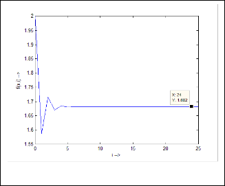
…value repeating

is the order of iteration. … (3.1)

In this case also if we consider as a random variable like all
the previous types, we get a result from (3.1), then the answer

again be considered as and so on. In this case, this series will
have a limiting value, which is
0·9998477415310881129598107686798 if we consider 31 digits


after decimal point. So,

(constant)
Ex.3.1: Now take an example: suppose we take any random variable  .
.
Then the iterative results will be:


0·92050485345244032739689472330046
0·99987094716081078813848034332851
0·99984773446360205953437286377479
0·99984774153324055527488336319716
0·99984774153108745742149048473084
0·99984774153108811315945862281788
0·99984774153108811295974996481155
0·99984774153108811295981078719796
0·99984774153108811295981076867416
0·9998477415310881129598107686798
0·9998477415310881129598107686798
…value repeating
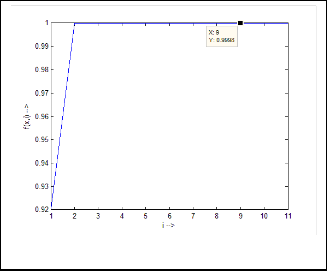
Fig.10. Output response of Ex.2.6
So prediction in (2.3) is also proved analytically.
Fig.11. Output response of Ex.3.1
IJSER © 2012
http://www.ijser.org
International Journal of Scientific & Engineering ResearchVolume 3, Issue 9, September-2012 8
ISSN 2229-5518
Ex.3.2: Take another example:  Then the iterative results will be:


–0·57357643635104609610803191282616
0·99994989238691479899521937732222
0·9998477104188857772677217602915
0·99984774154056350767740513976426
0·99984774153108522717546536452938
0·99984774153108811383869249723479
0·99984774153108811295954310034415
0·99984774153108811295981085019969
0·99984774153108811295981076865497
0·99984774153108811295981076867981
0·9998477415310881129598107686798
0·9998477415310881129598107686798
…value repeating
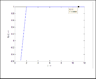
Fig.13. Output response of Ex.3.3
Then our prediction was exactly right. This is proved now by analytical method.
So, as we can see

Fig.12. Output response of Ex.3.2

Ex.3.3: Take another example:  The iterative results will be:


0·39073112848927375506208458888909
0·99997674699528153455312175786626
0·99984770223921958855808301788233
0·99984774154305467057989511316751
0·99984774153108446847789970519695
0·99984774153108811406975807530513
0·99984774153108811295947272803272
0·99984774153108811295981087163197
0·99984774153108811295981076864845
0·99984774153108811295981076867981
0·9998477415310881129598107686798
0·9998477415310881129598107686798
…value repeating

In this case we can say 

where = 0·9998477415310881129598107686798
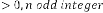
This type of series is not applicable for  , or other
trigonometric expression.

So, for  be the iterative function of random variable

and  be the order of iteration and is defined as


 , then
 constant.
So this is also an example of limiting progression.
2.4 Type IV


Limiting Progressive Function: Predicting Expression:
Form:


 is a value, not in
degree, is the order of iteration. … (4.1)

In this case also if we consider as a random variable, we get


a result from (4.1) for  iteration, then this value is again used as for
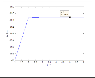
 iteration and so on. In this case also this series will have a limiting value which is 89·35883917 if we consider 8 digits after point. If be positive, the limiting value will be positive and if be negative, the limiting value
will be negative.
Ex.4.1: Now let’s take an example: 
Then the iterative results will be:


88·72696998
89·35427352
89·35880641
89·35883893
89·35883916
IJSER © 2012
http://www.ijser.org
International Journal of Scientific & Engineering ResearchVolume 3, Issue 9, September-2012 9
ISSN 2229-5518

89·35883917 
89·35883917 
…value repeating.
…value repeating
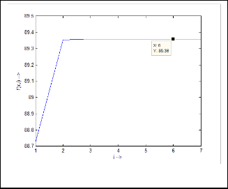
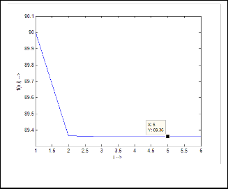
Fig.16. Output response of Ex.4.3
Fig.14. Output response of Ex.4.1
Ex.4.2: Take another example:  Then the iterative results will be:


89·99752331
89·36338891
89·35887181
89·3588394
89·35883917
89·35883917
…value repeating.
So, this prediction was true. As we can see
So, we can say where x = 89·35883917
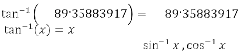
This type of series is not applicable for , or oth-
er inverse trigonometric expression.

So, for  be the iterative function of random variable

and  be the order of iteration and is defined as


 , then
 constant.
So this is also an example of limiting progression.
2.5 Type V
Limiting Progressive Function:


Predicting Expression:

Limiting Progressive Function:


Predicting Expression:

Fig.15. Output response of Ex.4.2


Form(I):

where

Ex.4.3: Take another example:  Then the sequential results will be:


–89·9975331
–89·36338891
–89·35887181
–89·3588394
–89·35883917
–89·35883917

 is the order of iteration. … (5.1)

In this case also if we consider as a random variable, we get

a result from (5.1) for  iteration, then this value is again used as for
 iteration and so on. In this case also this series will have a limiting value which is 0·017453292 if we consider 9 digits after decimal point.

Ex.5.1.1: Now consider an example: Let’s take 
The successive iterative results will be:
0·006818459 

IJSER © 2012
http://www.ijser.org
International Journal of Scientific & Engineering ResearchVolume 3, Issue 9, September-2012 10


ISSN 2229-5518
0·017453292
0·017453292
and thus so on.


In this case also if we consider as a random variable, we get a result from (5.2) for  iteration, then this value is again used as for
 iteration and so on. In this case also this series will have a limiting value which is 0·017453293 if you consider 9 digits after point.

Ex.5.2.1: Now consider an example: Let’s take 
The successive results will be:=


–0·012519227
0·017453292
0·017453293
and thus so on.
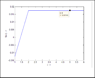
Fig.17. Output response of Ex.5.1.1
So, it is now clear that, this series has a limiting value:
0·017453292.

Ex.5.1.2: Now let’s take another example: 
The iterative results will be:


0·017452746
0·017453292
0·017453292
………
Fig.19. Output response of Ex.5.2.1
So, it is now clear that, this series has a limiting value
0·017453293.

Ex.5.2.2: Now let’s take another example: 
The iterative results will be:


0·017454384
0·017453293
0·017453293
………

Fig.18. Output response of Ex.5.1.2
Here also the limiting value is 0·017453292.
Actually this value is: 0·017453292250022980737699843973
considering 31 digits after decimal point.
Form (II):

 where
where 

 is the order of iteration. … (5.2)
IJSER © 2012
Fig.20. Output response of Ex.5.2.2
http://www.ijser.org
International Journal of Scientific & Engineering ResearchVolume 3, Issue 9, September-2012 11
ISSN 2229-5518
Here also the limiting value is 0·017453293.
Actually this value is:
0·017453293059783998466834689798considering 31 digits after
decimal point. However, we have seen than these limiting
values of those two series are about same (up to 8 digits after
decimal point).
Moreover  series has no such property.


So, for  be the iterative function of random variable and
  be the order of iteration and is defined as


 ,then
,then constant.
So these are also the examples of limiting progression. There are many other types of limiting progression.
3 APPLICATION OF LIMITING PROGRESSION IN THE CONTEXT OF TRANSFER FUNCTION OF A FEEDBACK SYSTEM


For type I: 
 ,
,  ,
,

, 
In reference with Ex.1.1: 
 ,
, 
 and
and  .
.

Here is the initial input and  are the consecutive inputs

and is the  -th output of the system. Again
  and are the independent parameters of the feedback system. Here the system is called the feedback system as the output is fully or partially used as input to the same system.
  is the trans- fer function of the feedback system.

Here from the iterative outputs of the system, it is clear that the limiting value (final value) does not depend on the input or the output of the system rather depends on the parameters of the system. So if we have only  and , we will have the fi- nal value of the system, whatever be the input of the system. So we can predict the system. In these two cases the predicted value is always 6.


We have another output parameter of the system which is  .
.  is equivalent to ‘time’ in time domain analysis of the system. Here the value of
  where the limiting value is attained, is not only depends on
  and but also the
  i.e. the input of the system. In reference with Ex.1.1 and Ex. 1.2, the value of
  and are same in both case i.e. 2 and 3 respectively. But while reaching the limiting value, the value of
  is 44 and 39 in the two different cases respectively, where the inputs were 2341 and 123.29 respectively. Hence we can conclude that the value
of  also depends on initial input of the system.
viz. 23 and 1345, but in both cases,  . We have seen that the limiting value of the progression is 2·828427125 in both cases.


Case (2): Here has a limitation while  , it should be odd always, because th root of a negative real number is always imaginary when is even integer. The rest of the conclusion is same.
Case (3): When 
 , the feedback system will have special characteristics. The system will be oscillatory in nature, but not like positive feedback. The limiting value will have the same amplitude both in positive and negative side of
  -axis (time axis). So this system will have marginal stability (much like sinusoidal in nature). As in Ex.2.5


 , the limiting value is ±2·828427125.
Case (4): When 
 , a single limiting value is attained, from both side of
  -axis. Initially the system will have a decaying oscillating nature, and gradually it will attain a limiting value. As described in Ex.2.6.


 , the system will attain a limiting value of 1·681792831 after passing through an initial decaying oscillation.


For type III: 


 , typeIV:
andtype V:


there is no independent parameter of these types of feedback systems.  is only acting as dependent parameter which is de- pendent only on
  i.e. the initial value of . These are all the examples of constant limiting progression, as whatever be the initial input condition, the final output of the system is always same. So we can’t control the output of these systems.
4 CONCLUSIONS AND FUTURE WORKS
Prediction of output and controlling of a system based on the prediction can be done using the mathematical study of the system. This study is not complete yet, as the expression of  where the limiting value is attained is not clear yet. As
  is de- pendent on the system parameter and the initial input value, so it must have an expression. Working on these expressions requires time domain analysis of the system. So this paper gives an initial concept and steps towards the mathematical study. All the software simulations are done in MATLAB.


For type II: 


Case (1): In reference with Ex.2.1: 

ACKNOWLEDGMENT
I wish to thank my college Future Institute of Engineering and Management for inspiring and encouraging me as an under- graduate engineering student.


In this case also, we can conclude in the same way through the essence of the previous discussion, that  and are acting as independent parameters of the feedback system and
  is acting as dependent parameter which is dependent on
  , and . As in Ex.2.1 we have discussed using different values of
REFERENCES
[1] F. Golnaraghi, B.C.Kuo, Automatic Control Systems, Ninth Edition, John Wiley & Sons Inc, 2010.
[2] A. K. Mandal, Introduction to Control Engineering, Modeling, Analysis
IJSER © 2012
http://www.ijser.org
International Journal of Scientific & Engineering ResearchVolume 3, Issue 9, September-2012 12
ISSN 222S-5518
and Design, New Age International Publishers, 2006.
IJSER lb) 2012
htt p://www .'lser. ora