International Journal of Scientific & Engineering Research, Volume 6, Issue 5, May-2015 1889

ISSN 2229-5518

MULTI-SAMPLE ADAPTIVE TEST AND OTHER COMPETITATORS IN LOCATION PROBLEM

1.1 Introduction:

If the parametric assumptions are fulfilled, classical F test is the appropriate test for the multi sample location problem. On the other hand, if assumptions not satisfies ,F-test is not a suitable tests. So we have to search for some other tests. Test based on ranks or scores are found to be more powerful and robust in many situations. It is seen that many of the practicing statisticians have no idea regarding the data type. In this situations, the adaptive tests based on Hogg’s concept , may help the statistician to identify data type with respect to some measures like skewness and tail weight and then to select an appropriate rank test or test based on scores for classified type of distribution. In this chapter, we have first discussed the adaptive test procedure that are used to select an appropriate test and then compare an adaptive test and some of the tests procedure s with the help of Monte Carlo simulation technique. Both empirical level and power of these tests are calculated and comparison are made with F-test and different other adaptive tests. We have observed that adaptive tests behave well in broad class of distributions.

1.2 Selection Statistics:

Here we will use a selection statistics S =(Q1 ,Q2 ), where Q1 and Q2 are Hoggs measure of skewness and tailweight defined by –
Q1 =

𝑈�5%−𝑀� 50%

𝑀� 50% −𝐿� 5%

and Q2 =

𝑈�5% −𝐿�5%

𝑈�50% −𝐿�50%

Where , 𝑈�5% , 𝑀�50% and 𝐿�5% are the averages of the upper 5% , middle 50% and lower 5%
of the order statistics of the combined sample. 𝑈�50% and 𝐿�50% are the averages of the upper
50% and lower 50% of the order statistics of the combined sample
Table 1.1: Theoretical values of Q1 and Q2 for some selected distributions-

IJSER © 2015 http://www.ijser.org

International Journal of Scientific & Engineering Research, Volume 6, Issue 5, May-2015 1890

ISSN 2229-5518

Now let us define four categories of S- D1 = {S/0≤Q1≤ R2, 1≤Q2 ≤2}
D2 = {S/0≤Q1 ≤2; 2≤Q2 ≤3}
D 3 = {S/ Q 1 ≥0; Q2 >3}
D 4 = {S/ Q1 >2; 1≤Q2 ≤3}
This means that the distribution is short or medium tails if S falls in the
Category D1 or D2 respectively; long tail if S falls in the category D3 and right skewed tail if it falls in the category D4
Buning (1996) proposed the following adaptive test A :
𝐺 𝑖𝑓 𝑆 ∈ 𝐷1
𝐴 = � 𝐾𝑊 𝑖𝑓 𝑆 ∈ 𝐷2
𝐿𝑇 𝑖𝑓 𝑆 ∈ 𝐷3
𝐻𝐹𝑅 𝑖𝑓 𝑆 ∈ 𝐷4

1.3 Test Procedures :

IJSER © 2015 http://www.ijser.org

International Journal of Scientific & Engineering Research, Volume 6, Issue 5, May-2015 1891

ISSN 2229-5518

Let 𝑋𝑖1 , 𝑋𝑖2 , … , 𝑋𝑖𝑛𝑖 , i =1,2,…,c be independent random variables with absolutely
continuous distribution function F(x-𝜃R i).
Here the null hypothesis H0 :𝜃1 = 𝜃2 = ⋯ = 𝜃𝑐
Against the alternative hypothesis H1 :𝜃𝑟 ≠ 𝜃𝑠 for at least one pair (r,s), r≠s.

1.3.1 F-Test:

For normally distributed random samples with equal variance, in testing equality of means the likelihood ratio F test is the best one. The test statistics defined as
F = (𝑁−𝑐) ∑𝑖=1

𝑛𝑖 (�𝑋�𝚤−𝑋� )2

∑ ∑𝑛

−𝑋 )

(𝐶−1)

𝐶

𝑖=1

𝑖 (𝑋𝑖𝑗

� �𝚤 2

where N=∑𝑐
𝑛𝑖 , 𝑋�
= 1
∑𝑛𝑖 𝑋
, 𝑋� =

1 ∑𝑐

𝑛𝑖 𝑋�𝑖

𝑖=1

𝑖 𝑛𝑖

𝑗=1

𝑖𝑗

𝑁 𝑖=1

Under H0 the test statistics follows F distribution with c-1 and N-c degrees of freedom.

1.3.2 Kruskal-Wallis(KW) test:

Let Rij be the rank of the observation xij in the pooled sample. The Kruskal- Wallis test for two-sided alternative which based on the statistic

KW =

12 ∑ 1 R

− ni ( N + 1) 

N ( N + 1) i =1 ni  2 

KW = 12
∑𝑐

1 [𝑅

- 𝑛𝑖 (𝑁+1) ]2

𝑁(𝑁+!)

𝑖=1 𝑛𝑖

𝑖 2 P

= 12
∑𝑐

2

𝑖 − 3(𝑁 + 1)

𝑁(𝑁+1)

𝑖=1 𝑛𝑖

where

ni

Ri = ∑ Rij

and N =∑𝑖=1 𝑛𝑖 .

j =1

IJSER © 2015 http://www.ijser.org

International Journal of Scientific & Engineering Research, Volume 6, Issue 5, May-2015 1892

ISSN 2229-5518

For sample size ni and sample number k large , H o is rejected if KW> χ 2
. When k is
small and ni are small then exact distribution table of KW can be used.
Now let us define linear rank statistics. Let us consider a the combined ordered sample 𝑋(1),𝑋(2),…. 𝑋(𝑁) of 𝑋11, … 𝑋1𝑛1,….𝑋𝑐1, … 𝑋𝑐𝑛𝑐 and indicator variables Vik given by
𝑉 = 1 𝑖𝑓 𝑋(𝑘) 𝑏𝑒𝑙𝑜𝑛𝑔 𝑡𝑜 𝑡ℎ𝑒 𝑖𝑡ℎ 𝑠𝑎𝑚𝑝𝑙𝑒 , 𝑖 = 1, … , 𝑐, 𝑘 = 1, … , 𝑁
0 𝑜𝑡ℎ𝑒𝑟𝑤𝑖𝑠𝑒
where N=∑𝑐
𝑛𝑖 ,
Let a(k) , k =1,2,…,N be real valued score with mean 𝑎� = 1 ∑𝑁
𝑎(𝑘). now we define for

𝑁 𝑘=1

each sample a statistics Ai in the following way:
Ai =

1

𝑛𝑖

𝑁

𝑘=1

𝑎(𝑘)𝑉𝑖𝑘, 1≤i≤c
Then the linear rank statistics LN is given by
LN =

(𝑁−1) ∑𝑐

𝑛𝑖 (𝐴𝑖−𝑎�)2

∑𝑁

(𝑎(𝑘)−𝑎�)2

𝑘=1

Under H0 ,LN is distribution free and follows asymptotically chi- square distribution with c-1 degrees of freedom .
Some of the scores to obtain more powerful test for types of distribution according to
Buning(1991,1994) are as follows:

1.3.3 Gastwrith test G (short tails ):

IJSER © 2015 http://www.ijser.org

International Journal of Scientific & Engineering Research, Volume 6, Issue 5, May-2015 1893

ISSN 2229-5518

⎧ 𝑘 −
⎪

(𝑁 + 1)
4
𝑖𝑓 𝑘 ≤

(𝑁 + 1)
4
𝑎𝐺 (𝑘) =
0 𝑖𝑓
⎨

(𝑁 + 1)
4
≤ 𝑘 ≤

3(𝑁 + 1)
4
⎪
⎩𝑘 −

3(𝑁 + 1)
4 𝑖𝑓 𝑘 ≥

3(𝑁 + 1)
4

1.3.4 Kruskal wallis test KW (medium tails):

If 𝑎𝐾𝑊 (𝑘) = 𝑘, test transform to above KW test

1.3.5 Test LT (long tails ):

𝑁
⎧ −(�
⎪ 4

𝑁
� + 1 𝑖𝑓 𝑘 < � 4
� + 1
𝑎𝐿𝑇 =
𝑘 −
⎨

(𝑁 + 1)
2

𝑁
𝑖𝑓 � 4
� + 1 ≤ 𝑘 ≤ [

3(𝑁 + 1)
4 ]
⎪ 𝑁
3(𝑁 + 1)


⎩ � 4 � + 1 𝑖𝑓 𝑘 > [ 4 ]

3.3.6 Hogg Fisher Randles test HFR(right skewed ):

𝑎𝐻𝐹𝑅 = �
𝑘 −

(𝑁 + 1)
2
𝑖𝑓 𝑘 ≤

(𝑁 + 1)
2
(𝑁 + 1)

0 𝑖𝑓 𝑘 > 2
For left-skewed distributions we change the terms k- (N+1)/2 and 0 in the definition of the scores above.

1.4 Monte Carlo simulation:

IJSER © 2015 http://www.ijser.org

International Journal of Scientific & Engineering Research, Volume 6, Issue 5, May-2015 1894

ISSN 2229-5518

We investigate the power of the tests via Monte Carlo simulation. For this purpose we have repeated 10000 times. The criteria of the test comparisons are the level 𝛼 and the
power 𝛽 of the tests. The concept of 𝛼 robustness can be defined as follows. For a nominal level 𝛼 and underlying distribution function F, the critical region 𝐶𝛼 of a statistic T may be uniquely determined by 𝑃𝐻0 (𝑇 ∈ 𝐶𝛼 ! 𝐹) = 𝛼. We now assume a distribution function for the data and determine the actual level 𝛼 ∗ of the test, i.e. 𝛼 ∗ = 𝑃𝐻0 (𝑇 ∈ 𝐶𝛼 ! 𝐺), T is then called
‘𝛼 − 𝑟𝑜𝑏𝑢𝑠𝑡’ if ! 𝛼 − 𝛼 ∗ ! is small. In case of 𝛼 ∗ ≤ 𝛼, we call the test conservative;
otherwise , it is anticonservative.
The selected distributions for the robustness and power study are Normal, Logistic, Cauchy, Lognormal, Double Exponential, Exponential and Uniform. We consider cases of three samples and Four samples with sample size combinations (10,10,10),(10,15,20), (10,10,10,10) and (10,15,20,25). Various combinations of location parameters are considered which are shown in respective Tables. For generating the samples from the normal distribution formula given by Hammersley and Hanscomb(1964 ) is used and for other distributions we have used method inverse integration. Necessary modification are made in generated sample to represent the location shift.

IJSER © 2015 http://www.ijser.org

International Journal of Scientific & Engineering Research, Volume 6, Issue 5, May-2015 1895

ISSN 2229-5518

Table 1.2 Empirical Level and power of tests under Normal distribution:

IJSER © 2015 http://www.ijser.org

International Journal of Scientific & Engineering Research, Volume 6, Issue 5, May-2015 1896

ISSN 2229-5518

Fig-1.1 Empirical power of tests under Normal distribution for n1 =n2 =n 3 =10

at 5% level:

1.0

0.8

0.6

0.4

0.2

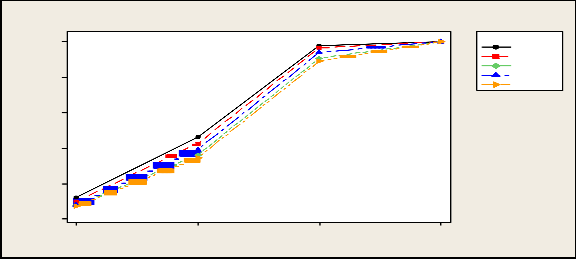
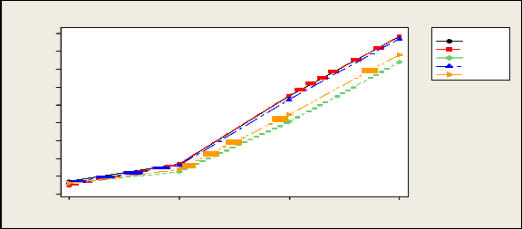
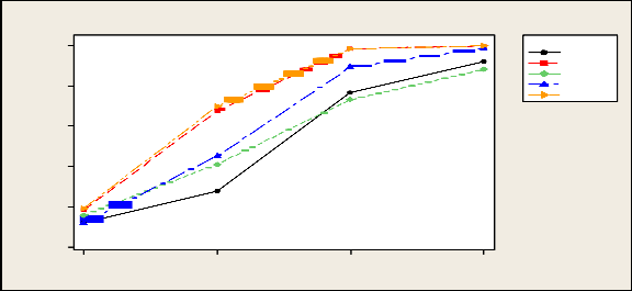
Empirical power of tests under Normal Dist.

Variable

F H G LT

HF R

0.0

(0,-.2,.2)

(0,-.5,.5)

means

(0,-1,1)

(0,-1.5,1.5)

Fig-1.2 Empirical power of tests under Normal distribution for n1 =10, n2 =15,

n3 =20, n4 =25 at 5% level:

1.0

0.8

0.6

0.4

0.2

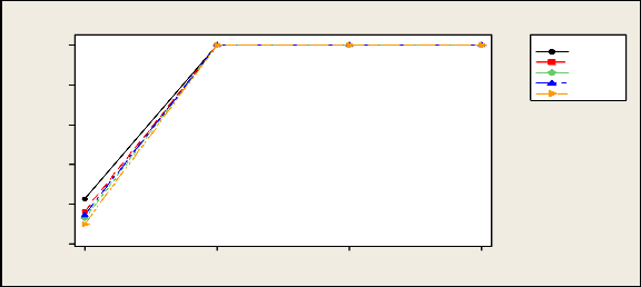
Empirical power of tests under Normal Dist.

Variable

F H G LT

HF R

0.0

(-.1,1,-.2,.2)

(-.5,.5,-1,1)

(-1,1,-1.5,1.5)

means

(-1.5,1.5,-2,2)

IJSER © 2015 http://www.ijser.org

International Journal of Scientific & Engineering Research, Volume 6, Issue 5, May-2015 1897

ISSN 2229-5518

Table 1.3 Empirical Level and power of tests under Cauchy distribution:

IJSER © 2015 http://www.ijser.org

International Journal of Scientific & Engineering Research, Volume 6, Issue 5, May-2015 1898

ISSN 2229-5518

Fig 1.3 Empirical power of tests under Cauchy distribution for

n1 =n2 =n 3 =10 at 5% level:

0.8

0.7

0.6

0.5

0.4

0.3

0.2

0.1

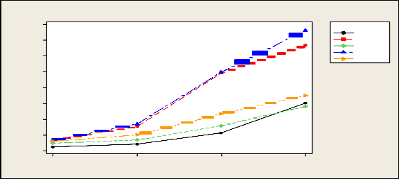
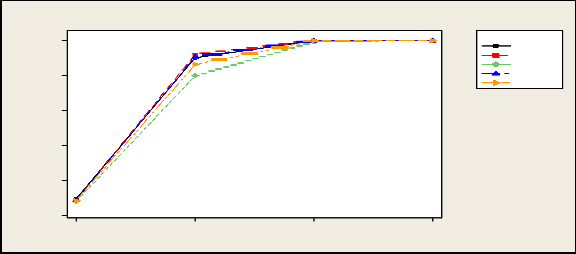
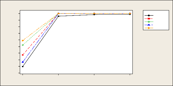
Empirical power of tests under Cauchy dist.

Variable

F H G LT

HF R

0.0

(0,-.2,.2)

(0,-.5,.5)

means

(0,-1,1)

(0,-1.5,1.5)

Fig.1.4Empirical power of tests under Cauchy distribution for n1 =10, n 2 =15,

n3 =20, n4 =25 at 5% level:

1.0

0.8

0.6

0.4

0.2

Empirical powerof tests under Cauchy dist.

Variable

F H G LT

HF R

0.0

(-.1,.1,-.2,.2)

(-.5,.5,-1,1)

(-1,1,-1.5,1.5)

means

(-1.5,1.5,-2,2)

IJSER © 2015 http://www.ijser.org

International Journal of Scientific & Engineering Research, Volume 6, Issue 5, May-2015 1899

ISSN 2229-5518

Table 1.4 Empirical Level and power of tests under Logistic distribution:

IJSER © 2015 http://www.ijser.org

International Journal of Scientific & Engineering Research, Volume 6, Issue 5, May-2015 1900

ISSN 2229-5518

Fig. 1.5 Empirical power of tests under Logistic distribution for n1 =n2 =n3 =10

at 5% level:

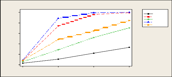
Empirical power of tests under Logistic dist.

0.9

0.8

0.7

0.6

0.5

0.4

0.3

0.2

0.1

Variable

F H G LT

HF R

0.0

(0,-.2,.2)

(0,-.5,.5)

means

(0,-1,1)

(0,-1.5,1.5)

Fig. 1.6 Empirical power of tests under Logistic distribution for n1 =10, n2 =15,

n3 =20, n4 =25 at 5% level:

1.0

0.8

0.6

0.4

0.2

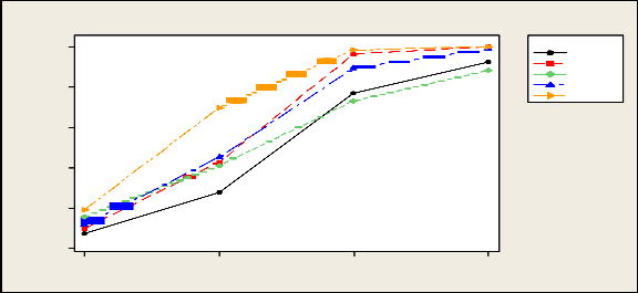
Empirical power of tests under Logistic distribution

Variable

F H G LT

HF R

0.0

(-.1,.1,-.2,.2)

(-.5,.5,-1,1)

(-1,1,-1.5,1.5)

means

(-1.5,1.5,-2,2)

IJSER © 2015 http://www.ijser.org

International Journal of Scientific & Engineering Research, Volume 6, Issue 5, May-2015 1901

ISSN 2229-5518

Table 1.5 Empirical Level and power of tests under Lognormal distribution:

IJSER © 2015 http://www.ijser.org

International Journal of Scientific & Engineering Research, Volume 6, Issue 5, May-2015 1902

ISSN 2229-5518

Fig. 1.7 Empirical power of tests under Lognormal distribution for n1 =n2 =n 3 =10

at 5% level:

1.0

0.8

0.6

0.4

0.2

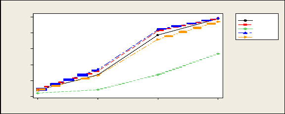
Empirical power of tests under Lognormal distribution

Variable

F H G LT

HF R

0.0

(0,-.2,.2)

(0,-.5,.5)

means

(0,-1,1)

(0,-1.5,1.5)

Fig. 1.8 Empirical power of tests under Lognormal test for n1 =10, n2 =15, n3 =20,

n4 =25 at 5% level:

1.0

0.9

0.8

0.7

0.6

0.5

0.4

0.3

0.2

Empirical power of tests under Lognormal distribution

Variable

F H G LT

HF R

0.1

1

2 3 4

means

IJSER © 2015 http://www.ijser.org

International Journal of Scientific & Engineering Research, Volume 6, Issue 5, May-2015 1903

ISSN 2229-5518

Table 1.6 Empirical Level and power of tests under Exponential distribution:

IJSER © 2015 http://www.ijser.org

International Journal of Scientific & Engineering Research, Volume 6, Issue 5, May-2015 1904

ISSN 2229-5518

Fig. 1.9 Empirical power of tests under Exponential distribution for n1 =n 2 =n3 =10

at 5% level:

1.0

0.8

0.6

0.4

0.2

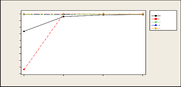
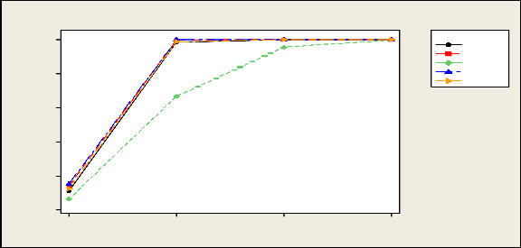
Empirical power of tests under Exponential dist

Variable

F H G LT

HF R

0.0

(0,-.2,.2)

(0,-.5,.5)

means

(0,-1,1)

(0,-1.5,1.5)

Fig. 1.10 Empirical power of tests under Exponential test for n1 =10, n2 =15, n3 =20,

n4 =25 at 5% level:

1.0

0.9

0.8

0.7

0.6

0.5

0.4

0.3

0.2

Empirical power of tests under Exponenetial dist

Variable

F H G LT

HF R

0.1

(-.1,.1,-.2,.2)

(-.5,.5,-1,1)

(-1,1,-1.5,1.5)

means

(-1.5,1.5,-2,2)

IJSER © 2015 http://www.ijser.org

International Journal of Scientific & Engineering Research, Volume 6, Issue 5, May-2015 1905

ISSN 2229-5518

Table 1.7 Empirical Level and power of tests under Double Exponential

Distribution:

IJSER © 2015 http://www.ijser.org

International Journal of Scientific & Engineering Research, Volume 6, Issue 5, May-2015 1906

ISSN 2229-5518

Fig.1.11 Empirical power of tests under Double Exponential distribution for

n1 =n2 =n3 =10 at 5% level:

Empirical power of tests under Double Expo. dist

1.0

0.8

0.6

0.4

0.2

Variab le

F H G LT

HF R

0.0

(0,-.2,.2)

(0,-.5,.5)

means

(0,-1,1)

(0,-1.5,1.5)

Fig.1.12 Empirical power of tests under Double Exponential distribution for n1 =10,

n2 =15, n3 =20, n4 =25 at 5% level:

1.0

0.8

0.6

0.4

0.2

Empirical power of tests under Double Expo. dist

Variable

F H G LT

HF R

0.0

(-.1,.1,-.2,.2)

(-.5,.5,-1,1)

(-1,1,-1.5,1.5)

means

(-1.5,1.5,-2,2)

IJSER © 2015 http://www.ijser.org

International Journal of Scientific & Engineering Research, Volume 6, Issue 5, May-2015 1907

ISSN 2229-5518

1.5 Discussion:

From Table 3.2 it is seen that empirical level of almost all tests satisfies the nominal level. In case of power , F- test seems to be more powerful than other tests followed by Kruskal –Wallis test. But as the location shift , sample size increases power of all the tests going to be almost equal.
In case Cauchy distribution, only Kruskal-Wallis and Long-tail test satisfies the nominal levels under the null situations. F-test not at all satisfies the nominal level. However,G, HFR slightly better than F-test. Power of Long –tail test (LT) seems to be the highest of all the tests discussed here.
Table 3.4 shows the empirical level and power of six tests under logistic distribution. Here we have observe that all the test satisfies the nominal levels. It is seen that power of F-test and Kruskal –Wallis tests are almost similar. However, KW tests are slightly higher in some situations. Out of three score tests, power LT test is higher than other two tests.
Table 3.5 shows the empirical level and power of tests under lognormal distribution. It is seen that except F –test all other tests satisfy the nominal level approximately. Here we have seen that power of HFR test is more than other tests. Power of F and G test are found to be less than other tests.
Table 3.6 shows empirical levels and powers of tests under exponential distribution . Here we have found similar results as lognormal distribution. Since both are right-skewed distribution that why we get similar results.
From 3.7 , we have found the empirical levels and power of the six tests. It is
observe that except G test, empirical level of other test are closed to nominal levels. It is also

IJSER © 2015 http://www.ijser.org

International Journal of Scientific & Engineering Research, Volume 6, Issue 5, May-2015 1908

ISSN 2229-5518

clear that power of LT test is the highest of all , followed by KW and F test and HFR
respectively.

3.6 Conclusions:

From the above results we can conclude that ,F test is suitable for the normal distribution. For log tailed distribution LT test and H test is more preferable than other test. G test is suitable for short tailed distribution and HFR test is preferable for the right-skewed distribution. From these results it is clear that prior information regarding the observation distribution help in choosing the appropriate test. So, adaptive procedure certainly help the practioner for appropriate test selection and help to arrive at right conclusion.

Bibliography& References:

Bean, R.(1974). Asymptotically efficient adaptive rank estimates in location models.,

Annals of Statistics,2,63-74

Buning, H.(1991). Robuste and Adaptive Tests . De Gruyter, Berlin .

IJSER © 2015 http://www.ijser.org

International Journal of Scientific & Engineering Research, Volume 6, Issue 5, May-2015 1909

ISSN 2229-5518

Buning, H.(1994). Robust and adaptive tests for the two –sample location problem.

OR Spektrum 16,33-39.

Buning, H.(2000).Robustness and power of parametric ,nonparametric, robustified and adaptive tests – the multi-sample location problem., Statistical Papers 41,381-407.
Buning, H.(2002). An adaptive distribution-free test for the general two-sample
Problem. Computational Statistics 17,297-313.
Bunning, H.(1996).,Adaptive tests for the c-sample location problem-the case of two- Sided alternatives’, Comm.Stat. –Theo. Meth. 25,1569-1582.
Bunning, H. (1999).,Adaptive Jonckheere-Type Tests for Ordered Alternatives.

Journal of Applied Statistics ,26(5),541-51

Buning, H. And Kossler,W.(1998).Adaptive tests for umbrella alternatives.,

Biometrical journal,40,573-587.

Buning, H. And Kossler,W.(1999). The asymptotic power of Jonckheere-Type tests for ordered alternatives. Asutralian and New Zealand Journal of Stagbtistics,41(1), 67-77.
Buning, H. and Thadewald,T.(2000). An adaptive two-sample location-scale test of
Lepage-type for symmetric distributions. Journal of Staistical

Computation and Simuation., 65,287-310.

IJSER © 2015 http://www.ijser.org

International Journal of Scientific & Engineering Research, Volume 6, Issue 5, May-2015 1910

ISSN 2229-5518

Freidlin, B. And Gastwirth, J.(2000).Should the median test be retired from general use? The American Statistician,54(3),161-164.
Freidlin, B.;Miao,W. And Gastwirth, J.L.(2003a). On the use of the Shapiro-Wilk test In two- stage adaptive inference for paired data from moderate to very heavy tailed distributions. Biometrical Journal 45,887-900.
Gastwirth, J.(1965).Percentile Modification of Two-Sample Rank Tests,Journal of theAmerican Statistical Association, 60(312),1127-1141.,
Hajek, J.(1962). Asymptotically Most Powerful Rank- Order Tests .Annuals of

Mathematical Statistics ,33,1124-1147

Hajek, J.(1970). Miscellaneous Problems of Rank Test Theory. In M.L.Puri , ed., Nonparametric techniques in Statistical Inference, Cambridge, Mass.: Cambridge University Press.
Hajek, J. ; Sidak, Z. And Sen, P.(1999). Theory of Ranks, 2nd edition. New York and
London: Academic Press .
Hall, P. And Padmanabhan, A.R.(1997). Adaptive inference for the two-sample scale
Problem’ ,Technometrics 39,412-422.
Hao, Li and Houser, D.(2012). Adaptive procedures for Wilcoxon -Mann –Whitney
Test.,Seven Decades of Advances.
Hill, N.J., Padmanabhan,A.R. and Puri, M.L.(1988). Adaptive nonparametric

IJSER © 2015 http://www.ijser.org

International Journal of Scientific & Engineering Research, Volume 6, Issue 5, May-2015 1911

ISSN 2229-5518

procedures and applications’, Applied Statistics,37,205-218. Hogg, R.V.; Uthoff, V.A., Randles, R.H., and Devenport, A.S.(1972): ‘On the
selection of the underlying distribution and adaptive estimation’ ,

Jour.Amer.Stat.Assoc.,67,597-600.

Hogg, R.(1967). Some Observations on Robust Estimation.Journal of the Amarican

Statistical Association,62,1179-86.

Hogg, R.(1974). Adaptive Robust Procedure: A Partial Review and Some Suggestions for Future Applications and Theory. Journal of American Statistical Association,69(348),909-23.
Hogg, R.V.(1976). A new dimension to nonparametric tests. Commun. Stat. Theo.

Methods,A5, 1313-1325.

Hogg, R., Fisher, D. and Randles, R.(1975). A Two-Sample Adaptive Distribution
Free Test. Journal of the American Statistical Association, 70(351),656-61.
Hogg, R.V. and Lenth, R.V.(1984). A review of some adaptive statistical techniques.

Communications in Statistics- Theory and Methods.,13,1551-1579. Hogg, R.V. and Randales, R.H.(1975). Adaptive distribution free regression

Methods. Technometrics17,399-408.
Hogg, R.V.(1982). On adaptive statistical inference. Communications in Statistics ,

IJSER © 2015 http://www.ijser.org

International Journal of Scientific & Engineering Research, Volume 6, Issue 5, May-2015 1912

ISSN 2229-5518

Theory and Methods. ,11, 2531-2542.

Huber, P.J.(1972). Robust Statistics: A Review, Annals Math. Stat. ,43,1041-1067. Jaeckel Louis A.(1971).Robust Estimates of Location: Symmetry and Asymmetry
Contamination, Annals of Mathematical Statistics, 42,1020-34
Jones, D.(1979).An Efficient Adaptive Distribution Free Test for Location. Journal of the American Statistical Association., 74(368),822-28
Kossler, W. (2010). Max-type rank tests, U- tests and adaptive tests for the two
sample location problem- An Asymptotic Power Study. Computational

Statistics and Data Analysis.54(9),2053-2065

Kossler W. and Kumar N.(2008). An adaptive test for the two- sample
location problem based on U- statistics, Communications in Statistics- Simulation and Computation,37(7),1329-1346...
Kumar, N.(1997). A Class of Two-Sample Tests for Location Based on Sub-Sample
Medians. Communications in Statistics. Theory and Methods, 26,943-
951.
Mann, H. and Whitney, D. (1947).On a Test of Whether One of Two Random Variables is Stochastically Larger than the Other, Annals of Mathematical Statistics . 18(1),50-60.
Neuhaser, M., Bunning, H. and Hothorn, L.A.(2004). Maximum Tests versus

IJSER © 2015 http://www.ijser.org

International Journal of Scientific & Engineering Research, Volume 6, Issue 5, May-2015 1913

ISSN 2229-5518

Adaptive Tests for Two-Sample Location Problem’, Journal of Applied

Statistics.,31,215-227.

Neuhaeuser, M and Hothorn, L.A. (2005). Maximum tests are adaptive permutation
Tests., Journal of Modern Applied Statistical Methods, 5,317-322
O’Gorman, T.W.(1996). An Adaptive Two-Sample Test based on Modified Wilcoxon
Scores’, Communications in statistics. Simulation and. Computation,
25(2)459-479.
O’Gorman, T.W.(1997). A comparison of an adaptive two-sample test to the t-
test, rank-sum and log-rank tests, Commun. Statist. Simul. Compu., 26,1393-
1411.
O’Gorman, T.W.(2001). An adaptive permutation test procedure for several common tests of significance’, Computational Statistics and Data Analysis, 35,
335-350.
Policello, G.E.and Hettmansperger, T.P. (1976). Adaptive robust procedures for the one-sample location problem. Journal of the American.

Statistical. Association.,71,624-633.

Randles, R.H. and Hogg, R.V.(1973). Adaptive distribution-free tests, Comm. In

Statist.,2,337-356.

Randles, R.H. and Wolfe, D.A.(1979). Introduction to the Theory of Nonparametric

IJSER © 2015 http://www.ijser.org

International Journal of Scientific & Engineering Research, Volume 6, Issue 5, May-2015 1914

ISSN 2229-5518

Statistics, N.Y. Wiley, New York.

Ramberg, J., and Schmeiser, B.W. (1974). An Approximate Method for Generating
Symmetric Random Variables’, Communications of the ACM,17,78-82
Ruberg, S.J.(1986). A continuously adaptive nonparametric two-sample
Test’.Communications in Statistics, Theory and Methods, 15,2800-2920. Uthoff, V.A. (1970). An Optimum Test Property of Two Well-Known Statistics’,

Journal of the American Statistical Association,,65,1597-1600. Wilcoxon, F. (1945). Individual Comparisons by Ranking Methods’, Biometrics

Bulletin,1(6), 80-83.

***************************

IJSER © 2015 http://www.ijser.org

International Journal of Scientific & Engineering Research, Volume 6, Issue 5, May-2015 1915

ISSN 2229-5518

IJSER © 2015 http://www.ijser.org